Heat networks are a method of delivering heat to multiple properties via a fluid-filled pipe network from a single source of thermal energy. They are a key strategic technology for meeting Scotland’s greenhouse gas emissions reductions targets and consideration of the potential for heat networks in an area is a core requirement for local authorities’ Local Heat and Energy Efficiency Strategies.

Low-temperature heat networks draw thermal energy directly from the ground, bodies of water or from waste heat generated by, for example, industrial activities. The temperature in the pipes is lower than in a traditional heat network and it is upgraded at each individual property served by the network via a heat pump so it can be used for heating and hot water. Traditional heat networks generate thermal energy at a central energy centre, for example through the simultaneous generation of electricity and heat from a gas-fired power station, and deliver it at a higher temperature to individual properties where the heat doesn’t need to be upgraded.

To date, most local and national energy planning in Scotland has focused on higher temperature heat networks. This research aims to support policies, strategies and delivery plans, locally and nationally, by showing where the opportunities low-temperature heat networks are likely to be strongest across Scotland.

Key findings

• There are low-temperature heat network opportunities in each of Scotland’s 32 local authority areas.
• While opportunities are concentrated in more heavily populated regions, such as the Central Belt and urban areas around Aberdeen and Dundee, opportunities can be found in the majority of Scotland’s towns, as well as in rural and coastal villages.
• About a third of Scotland’s housing stock and a third of non-domestic properties – around 1 million properties – could be served by low-temperature heat networks.
• Opportunities are split by those that could serve multiple buildings (11,000 opportunities) and those that could serve single buildings containing multiple individual properties such as block of flats (17,000).
• The majority of opportunity groupings involve modest numbers of properties (up to 30) and total heat demand (up to 300 megawatt-hours per year). However, some groupings have much larger total heat demands, especially if they include anchor loads like hospitals and higher education buildings.
• The majority of opportunity groupings were matched with one or more nearby green spaces that could potentially host hidden heat-collecting boreholes. A smaller proportion was matched with nearby water bodies.

For further information, please read the report.

If you require the report in an alternative format, such as a Word document, please contact info@climatexchange.org.uk or 0131 651 4783.

Research completed: March 2026

DOI: https://doi.org/10.7488/era/7027

Executive summary

Background

Heat networks use fluid-filled pipes to carry thermal energy from one place to another, serving multiple end users.

Traditional heat networks typically feature an ‘energy centre’ where high temperature heat is generated before it is sent out to the heat-using properties which are connected to the network. By contrast, low temperature heat networks connect two or more properties to a shared source of thermal energy, without a central station where high temperatures are generated. Instead, heat pumps within individual properties or buildings extract heat from the network, which typically operates at less than 35 degrees centigrade, and upgrade it to provide heating and hot water.

Heat networks are identified as a key strategic technology for meeting Scotland’s greenhouse gas emissions reductions targets (Scottish Government, 2022). Assessing their potential is a core requirement for local authorities’ Local Heat and Energy Efficiency Strategies (LHEES), the first versions of which were published in 2023 and 2024.

To date, most local and national energy planning in Scotland has focused on high temperature heat networks, typically operating at more than 65 degrees centigrade. This research addresses that gap by identifying where low temperature heat network are most likely to be suitable.

Aims

The results of this assessment identify where low temperature heat networks are most likely to be suitable across Scotland.

The results can support a range of uses, including local and national energy planning, project identification and prioritisation, public engagement (including awareness-raising), business planning and strategy development, knowledge-building and as an input to future research. The intended users include the Scottish Government, local authorities, energy system planners, enterprise development agencies, heat network developers, social landlords, researchers and members of the public.

The approach that has been developed also has policy value. It provides a tested and documented methodology that can be repeated and refined in future assessments.

This is a national level, first pass assessment of locations where low temperature heat networks may be suitable. It does not assess the relative attractiveness or feasibility of specific opportunities. Instead, the data outputs provide data that users can apply to screen and prioritise opportunities according to their own objectives.

Findings

Figure 1 provides an overview of the methodology used in the assessment:

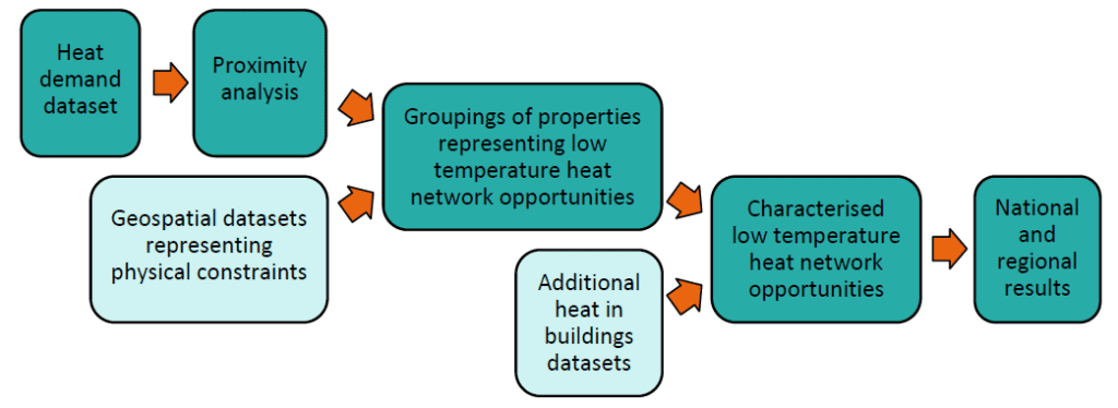
Figure 1: Simplified representation of national assessment methodology

In many areas, the most effective approach is likely to involve several smaller low temperature networks rather than a single large network. In denser urban locations, particularly in city centres, there are often multiple possible configurations. The opportunities identified should therefore be interpreted as areas of high potential rather than clearly defined project proposals.

The national assessment does not account for existing low temperature heat networks, recent or planned new build developments, networks that rely on both heating and cooling, or schemes involving large distances between buildings. To maintain a manageable and practical set of data outputs, smaller opportunities below a defined scale threshold were excluded. However, smaller low temperature heat networks connecting only a few properties can still be viable.

The assessment identified around 11,000 Multi-Building Opportunities and 17,000 Communal Opportunities across Scotland. Together, these represent approximately 900,000 domestic properties and around 100,000 non-domestic properties, around a third of each total. The heat demand represented by these opportunities combined amounts to over 20 TWh/yr.

• Most opportunities involve relatively small numbers of properties, typically up to 30, with total heat demand of up to 300 megawatt-hours per year. A smaller number of opportunities have much higher total heat demand, especially where anchor loads such as hospitals and higher education buildings are present.
• Low temperature heat network opportunities are distributed across each of Scotland’s 32 local authority areas. While concentrations are highest in more densely populated regions, including the Central Belt and urban areas around Aberdeen and Dundee, opportunities are also present in smaller towns, rural areas and coastal communities across Scotland.
• Most opportunities were matched with nearby green spaces that could potentially host heat collection infrastructure. A smaller proportion were matched with nearby water bodies, and relatively few with nearby waste heat sources, although, in some cases these offer significant potential.
• More than half of all opportunities are in areas where over 90% of properties currently use mains gas for heating. However, a notable proportion, around 16%, are located in areas with no mains gas use, often in off-gas locations or electrically heated buildings.

Recommendations

Scottish local authorities and other organisations involved in energy planning can use the results of the national assessment to inform strategies and delivery plans relating to heat networks, heat decarbonisation, and electricity network upgrades.

Organisations involved in project identification, including building owners, heat network project developers, community groups and economic development agencies, can use the datasets to screen and prioritise opportunities for further assessment. In some cases, access to the datasets will require compliance with data sharing agreements.

Confidence in the results of the national assessment could be improved through better evidence on the relationship between heat demand and viable connection distances between properties. Improvements to input datasets, particularly relating to heat demand and waste heat sources, would help to better capture the full potential for low temperature heat networks.

Glossary / Abbreviations

Low temperature heat networks

Just as electricity networks use cables to transport electrical energy from one or more points of generation to multiple points of use, heat networks use fluid-filled pipes to carry thermal energy from one place to another. Heat networks can take different forms. An important distinction that can be made between two of the main types relates to the temperature at which they operate. The temperature of the pipe network relative to the temperatures required by the end users has a fundamental impact on what items of equipment are required where on the network.

(a)

(b)

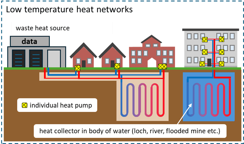
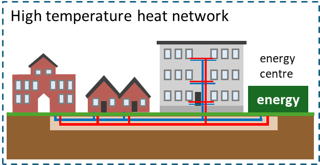
Figure 2: Simplified diagram of a) low temperature heat network features and b) high temperature heat network features

Figure 2 a) shows a simplified depiction of the features of low temperature heat networks. In each of the two networks shown, water-filled pipes connect separately occupied properties to a shared source (or sources) of thermal energy. The left network accesses thermal energy from a waste heat source (a data centre) as well as the ground and distributes it to separate buildings. The right network accesses a single heat source (a body of water) and distributes it to flats within a single building. The temperature of the water in the network is likely to be between 0 and 35 degrees centigrade (although could be warmer). In both instances, heat pumps in individual properties upgrade the temperature of the thermal energy that they extract from the network to supply space heating and hot water to occupants. Some low temperature heat networks are able to supply cooling to buildings in addition to (and often at the same time as) supplying heating.

By contrast, the high temperature heat network shown in Figure 2 b) shows multiple properties being supplied from a central energy centre. The temperature of the water that circulates from the energy centre to the end users is likely to be above 55 degrees centigrade, possibly much hotter. Connected properties do not normally need their own heat pumps. Instead, heat exchangers transfer thermal energy from the network to properties’ internal heating systems without upgrading its temperature.

Aims of the research

Policy value of the research outputs/

This national assessment of low temperature heat network opportunities aims to support the Scottish Government’s priority to reduce greenhouse gas emissions in the building sector. More specifically, it aims to support national and local policies, strategies and delivery plans associated with the development of low carbon heat networks in Scotland. It does this by providing the results of the first national-scale assessment of a class of heat networks that has, to date, typically been underrepresented in local and national energy planning. The results of the assessment show where low temperature heat networks are most likely to be suitable and provides additional data for each identified location that further characterises the opportunity. Aggregating the individual opportunities identified gives an indication of the extent and distribution of the overall opportunity for this type of heat network in Scotland.

The approach developed to generate these results itself also has value for policymakers and Scottish local authorities. Future assessments will be able to repeat and/or build on a tested, refined and documented methodology that has been designed with replicability in mind.

In addition to a policy and local government audience, it is anticipated that this research will have value for the heat network and heat-in-buildings industry, the owners and occupants of buildings that require heat decarbonisation solutions, energy network planners and operators, potential investors in heat networks, community organisations and interested members of the public.

This report communicates some of the results of the national assessment in the form of summaries relating to the low temperature heat network opportunities identified. This assessment is intended to inform decision making and does not determine the feasibility of individual projects.

Another critical output of the research is several datasets which capture details about the opportunities identified. Different versions of these geospatial datasets enable sharing with different recipients, depending on their organisation’s status (public sector or not) and the licenses that they hold to certain data products. The different versions enable users to gain maximum value from the research within the constraints imposed by data restrictions.

Context for interpretation

The national assessment is a top-down, “first pass” assessment of locations likely to be suitable for low temperature heat networks in Scotland. The opportunities identified in the research outputs have not been subject to any individual assessments. The selection process made use of information from national-scale datasets only; more localised information was not taken into account. Assessment of the relative attractiveness of specific opportunities was not within our scope.

The identified opportunities are entirely independent of the LHEES developed for each of Scotland’s 32 local authority areas. Local authorities have not carried out any screening of low temperature heat network opportunities ahead of publication. However, the research outputs offer important value for future development and the delivery of actions that align with them, particularly where local authorities are able to screen and prioritise opportunities relevant to their geographic area. This national assessment supplements, but does not supersede LHEES, it is intended to complement, rather than replace, LHEES.

The level of detail with which low temperature heat network opportunities were assessed is very much less than would typically be involved in a feasibility study. In most cases, the level of detail falls short of that which would typically be used to justify carrying out a feasibility study. Organisations wishing to pursue the assessment and possible development of a low temperature heat network in a specific location are advised to use the results of the national assessment as a starting point for a further investigation that incorporates local information. Users will need to apply judgment to develop and refine the concept for the network beyond the initial spatial boundary and the associated group of properties that are defined through this research.

The results of the national assessment inevitably include as “opportunities” some areas which are not in practice good locations for low temperature heat networks. They also fail to include some locations which would, upon further investigation, prove to be good opportunities. The national assessment can only offer generalised justifications for why a location has been included and another location excluded.

It is frequently the case that a group of properties that has been designated as a low temperature heat network opportunity would also represent an opportunity for a small high temperature heat network. The advantages and disadvantages of low temperature systems are often place-specific, requiring an options assessment to be carried out to establish which is likely to be a better fit for the heat sources, buildings and intermediate spaces involved.

Research concept and technical focus

Low temperature heat networks use a system of fluid-filled pipes to connect two or more buildings or separately occupied properties to a shared source of thermal energy. Low temperature heat networks, in common with many higher temperature networks, harvest energy from sources that are cooler than the temperatures needed by the buildings and processes they serve. Examples of these cooler heat sources include the ground, water bodies, and many waste heat sources. In contrast to higher temperature heat networks, these low temperature systems do not upgrade the temperature centrally – instead, one or more dedicated heat pumps per property supply the heating and hot water that the connected buildings need. Some low temperature heat networks are able to supply cooling to buildings in addition to (and often at the same time as) supplying heating.

In theory, low temperature heat networks could be used to heat buildings almost anywhere; all it takes is two or more buildings or separately occupied properties to be close enough together for it to make sense to share a heat source. However, some places are better than other places. This research aims to identify locations across Scotland where low temperature heat networks are most likely to be suitable. It aims to make available information about these locations and the opportunities there to facilitate consideration of low temperature heat networks as an option for decarbonising heat in buildings. This information includes the possible presence of waste heat sources near to heat network opportunities.

The opportunities identified could each be developed as a potential low temperature heat network scheme. However, it could be the case that smaller schemes within the areas delineated are more viable in practice – or that upon further investigation it makes sense to extend networks to certain neighbouring buildings outwith the areas mapped or to interconnect opportunity areas. The opportunities mapped and listed in the national assessment should be interpreted as guides to areas of high potential rather than defined proposals for schemes. For example, neither indicative pipe network routing nor precise locations for connections to heat sources are produced.

Use cases

The intended audience for the research comprises numerous groups who have the potential to contribute to meeting Scotland’s targets for building decarbonisation and heat network deployment. The degree to which the needs of the intended audiences for the research outputs are met is key to its impact. Therefore, the anticipated use cases are central to the aims of the research. This report aims to present the research and its results in such a way that readers can easily understand its implications and the conclusions reached. The data outputs produced by the research can be used for purposes that include local and national energy planning, project identification and prioritisation, public engagement (including awareness-raising), business planning and strategy development, knowledge-building and as an input to future research.

Scottish local authorities are a particularly important audience for the research. Having developed their LHEES over the period 2022 – 2024, local authorities are now engaged in implementing the Delivery Plans associated with the Strategies. In general, low temperature heat networks were not considered in detail when most of the Strategies and Delivery Plans were written. This outcome results from the methodology that local authorities were encouraged to follow when developing their LHEES in 2022 – 2024, which centred on high temperature heat networks. However, they have the potential to make a significant contribution to the decarbonisation of heat in buildings, alongside the other leading solutions:

• building energy efficiency;
• high temperature heat networks;
• individual, non-networked heat pumps; and
• other important technologies which have less widespread applicability.

The national assessment raises the profile of low temperature heat networks as a means to achieve the objectives of LHEES, and delivers information that can help local authorities (and other users) to focus on priority areas and to rank the opportunities that have been identified. Local authorities and their partners will still need to consider what the best technology choice is for each type of building in each locality. The national assessment does not directly compare low temperature heat networks against other zero-emissions heating solutions or identify optimum solutions, and as such cannot be a direct input into Delivery Plans or derived activities.

Other audiences that we specifically considered included:

• energy system planners;
• enterprise development agencies;
• heat network developers;
• social landlords;
• researchers; and
• members of the public, including those who are active in community organisations.

Developers of small high temperature heat networks may find that the results of the national assessment of low temperature heat network opportunities offer information that is useful for the identification of opportunities for higher-temperature systems. This would especially be the case if the results were combined with information about buildings’ temperature requirements and the density of heat demand at street-by-street level.

Our aim has been for the outputs to correlate as well as possible with real-world opportunities, while avoiding modelling factors that influence viability in subjective rather than objective ways. The national assessment acknowledges, and allows space for the influence of, local complexity while delivering a single assessment for the whole of Scotland.

Non-technical objectives

Non-technical objectives for the national assessment included:

• Geographic inclusivity – giving all areas of Scotland an equal ‘chance’ when it came to the identification of opportunities, after heat demand distribution is taken into account.
• Technical inclusivity – representing a range of possible scales, heat sources and network archetypes that can form viable low temperature heat networks.
• Replicability – developing a methodology that can be followed by others in the future to update results and further heat decarbonisation objectives.

Elements excluded from the national assessment

Table 1 lists the main types of low temperature heat network opportunity that are excluded from the national assessment for reasons of data unavailability, output useability, dependence on local energy planning outcomes and/or the need for focus on ‘mainstream’ and lower-risk opportunities.

Table 1: Summary of elements known to be excluded from the national assessment

Summary of methodology

This section summarises how the assessment identifies and characterises potential opportunities for low temperature heat networks.

The methodology for the national assessment was not developed in isolation. Several opportunities were created for stakeholders to consider and provide feedback on the methodological approach and many of the most influential decisions that were made. Stakeholder engagement covered the ways that information is presented and concepts communicated, in addition to the analytical processes that produce information outputs.

This chapter summarises the methodology in non-technical language, focusing on the concepts used rather than the sequential actions performed. Limitations of the research are discussed at the end of this chapter. Fuller detail of the methodological approach, justification of the decisions made, and the steps executed is set out in Appendix A.

The key data sets used as inputs were the Scotland Heat Map 2022, Home Analytics v4.1, Non-Domestic Analytics v2.0 and Green Heat in Greenspaces, supported by various Ordnance Survey and open government datasets. Input datasets were assessed in terms of data quality and the risks associated with uncertainty and inaccurate data. Where required, mitigating actions were taken. Mitigating responses included imposing limits on the influence of outlier heat demands and grouping quantitative data into bands to address concerns regarding the data’s consistency between different parts of Scotland.

The key outputs are geospatial polygons and point data that represent low temperature heat network opportunity locations, as well as some other features that help to enrich the understanding of the opportunities. Values in the datasets produced were aggregated to produce national and local summary results. Visual presentations of the data outputs were developed to enrich their interpretation and make them accessible to a wider audience.

The main steps followed included:

• Proximity analysis using a large dataset of potentially suitable heat demands and their relative locations – resulting in groupings of nearby heat demands;
• Application of constraints such as physical barriers and the size of the opportunities identified – resulting in geospatial features that represent Communal Opportunities, Multi-Building Opportunities and High Property Count Areas;
• Characterising opportunities via integrating additional datasets and performing calculations which aggregate information relating to all the heat demands within each opportunity – resulting in datasets that enrich the geospatial features.

The methodology aimed to identify clusters of heat demands that correlate reasonably well with real-world opportunities for low temperature heat network deployment but aimed to minimise the influence of more subjective assumptions. This means applying a relatively small number of selection criteria in the proximity analysis and constraints application stages but attaching a much wider range of informative attributes to the groupings once they had been created. Attributes selected included (among other parameters) property tenure, existing heating fuel usage and existing heating systems. The attribute selection responded to user needs as expressed in stakeholder consultations. The geospatial data presentations give users the ability to zoom in on specific places and see information that helps them to investigate which buildings are likely to be able to connect to a network and which ones aren’t. The appended information will help stakeholders to understand how good a particular opportunity is compared to all the others in their region or in the whole country, according to their own views on what makes an opportunity ‘good’. Users can also filter the long list of opportunities in order to only focus on those which possess certain characteristics, such as those located in regions of more constrained electrical grid capacity or those featuring a certain percentage of properties which are electrically heated.

Quality assurance of the methodology and the assumptions made was carried out by the researchers, and separately by Scottish Government representatives. A more detailed description of quality assurance checks is provided in Section 6 of Appendix A.

Heat demand proximity analysis

At a nationwide scale, three elements make more difference than anything else to the strength of an opportunity for low temperature heat networks:

• how close buildings or properties are together;
• whether buildings are divided into flats and other types of units like shops; and
• how much heat is needed by the properties.

The Scotland Heat Map dataset provides information on the locations of almost every building in Scotland, along with an estimate of how much heat each property needs (or in some cases, the heat it actually uses). To identify places where these elements come together in promising ways, we converted each property’s heat demand into a spatial distance proxy, representing the distance over which it may be viable to connect to neighbouring properties. The proxy represents an estimate of the real-world distance over which it could be viable for that property to share heat network infrastructure with a neighbour or neighbours. We designed a process that identifies when two or more properties’ proxy distances overlap, a circumstance that indicates that they could be part of the same low temperature heat network opportunity. This process generates many groupings of heat demands, each of which is reasonably ‘heat dense’.

Building inclusion and exclusion

Estimates for the heat demand of almost every building in Scotland are contained in the Scotland Heat Map (SHM). We removed around 10% of the heat demands from the dataset because they are unlikely to be able to benefit from a low temperature heat network connection:

• all heat demands less than 5,000 kWh per year (for which another zero-emissions heating system is likely to be lowest cost); and
• non-domestic heat demands with building use classifications that indicate a high likelihood that their heat demand is dominated by temperature requirements that exceed those which can normally be produced through networked heat pumps, or that are likely to have minimal or no heat demand. The list of excluded use classes is reported in Table 16 in Appendix A, Section 4.3.1.

We also removed heat demands which had been marked as likely to have issues in the dataset (for example, if the creators of the dataset considered that a building’s use classification indicated that it would not be expected to have a heat demand). The remaining SHM heat demand estimates were used for the calculation of the maximum connection distance for each of around 2.5 million properties in Scotland.

Domestic buildings’ suitability for networked heat pumps was not used as a criterion for excluding any heat demands from the analysis. It was assumed that there is a route to heat pump suitability for almost all domestic buildings. Where modifications are required (and in many instances they are not) they can include energy efficiency improvements and/or the upgrading of radiators and other types of heat emitter. High temperature ground source heat pumps (those able to output heat at more than 65°C) are an alternative way to successfully heat more challenging dwellings via low temperature heat networks.

Similarly, it was assumed that non-domestic buildings using energy for space heating and hot water generation are also almost always potentially suitable for connection to a low temperature heat network.

No screening was carried out by local authorities or other project partners.

Constraints on opportunity size and network reach

Our process mapped certain features of the physical world which are difficult and expensive for heat networks to cross – things like rivers, railways and big roads – so that they can exert constraints on how heat demands are grouped together into ‘opportunities’.

We determined that the national assessment would only map and characterise opportunities where at least ten homes could be connected to a network, or five buildings or units that are not homes. If there is a combination of homes and other types of property, a formula that weighs them up:

However, it is important to understand that low temperature heat networks can still be a good idea for smaller groups of buildings. A review of 34 operational Shared Ground Loop schemes in the UK (Barns et al., 2026) found that 13 of 34 (38%) schemes connected fewer than 20 heat pumps, with the minimum number of heat pumps being two. The restriction on size adopted in this research ensured that the number of opportunities identified was large but reasonable but does not imply that smaller schemes do not represent opportunities.

When identifying spatially dispersed opportunities, we made sure that the distance between buildings within an opportunity area does not risk being unrealistically large (while recognising that in exceptional circumstances, connections exceeding the 1 km threshold adopted could be feasible).

Distinct types of opportunity

An important distinction between two types of low temperature heat network concerns the number of buildings which are served by the network. Our process separated ‘Communal Opportunities’ (blocks of flats, tall tenement buildings and large multi-occupancy commercial buildings) from opportunities that consist of clusters of separate buildings.

Some areas in Scotland are particularly ‘heat dense’ – either they have a great number of heat demands close together, or there are multiple buildings present that demand especially large quantities of heat. Often both of these circumstances are present. These areas cover many of Scotland’s city centres and the centres of larger towns; they are also sometimes found in industrial areas or around very large hospitals. These areas often have significant overlap with the areas that have previously been identified as promising for the development of high temperature heat networks. Many options are likely to exist regarding the types and sizes of low temperature scheme that could be built within heat-dense zones. For example, a single large scheme could be viable – but it may also be possible to develop multiple smaller schemes or to develop in phases.

The proliferation of options for both high and low temperature heat networks means that it is particularly important that strategic energy planning is carried out before decisions are made about what should be built where. To avoid implying that any one technological solution is best within the more heat dense zones, and to recognise the possibility that many separate schemes could be developed within those areas, we separated them from smaller Multi-Building Opportunities. This was done simply on the basis of the number of heat demands (above or below 1,000). These areas with over 1,000 heat demands were referred to as High Property Count Areas (HPCAs).

It was found that the total heat demand of all properties within some HCPAs exceeded 100,000 MWh per year. This sub-group was referred to as High Heat Demand Areas. No Multi-Building Opportunities had total heat demands exceeding 100,000 MWh per year. Therefore, all High Heat Demand Areas were also High Property Count Areas.

Characterising opportunities

The previously described process of heat demand proximity analysis, barrier mapping, and opportunity classification generates a list of places where there are likely to be good prospects for constructing a low temperature heat network. (Whether or not a low temperature heat network is the best solution to decarbonising heat in that place has not been assessed through this research.) These places can be depicted on a map of Scotland or of a smaller area within Scotland, showing them either as singular points, as spatial areas or as indicators of the number and/or density of opportunities within a larger area.

In addition to the locations of opportunities, stakeholders have interest in other aspects of the spatial areas that they represent, the buildings within them and the people that live and work there. We researched what is most important for stakeholders through information-gathering workshops and a questionnaire. Wherever possible the data that is expected to be most valuable has been appended to the spatial datasets of opportunities such that a specific opportunity in a specific place is richly characterised. We generated quantitative summaries of the characteristics of opportunities across different geographical groupings, including the whole country and each local authority area.

Much less detailed characterising information was calculated for High Property Count Areas and High Heat Demand Areas than was the case for Multi-Building Opportunities. This choice reflects the fundamental difference between how larger and smaller opportunity groups should be approached. For larger groupings, including High Property Count Areas and High Heat Demand Areas, detailed local energy planning is essential to establish which low temperature heat network options exist and how they compare to other options. Furthermore, the large number of demands present in these areas means that aggregated information is less relevant and meaningful as an indicator of the characteristics of potential low temperature heat network schemes than is the case for smaller groupings of properties.

Linking heat sources to opportunities

A viable heat source for low temperature heat networks is present in almost all locations in Scotland. Closed loop boreholes are near-universally feasible and can be considered to be the default heat source for any of the opportunities identified (while recognising that space constraints may limit the amount of heat that can be extracted and supplied to a network). Open loop boreholes are less widely feasible but can offer significant advantages over closed loop boreholes. Often ground heat collectors of either type can be installed in close proximity to the heat demands connected to the network. In some circumstances, it can be beneficial to construct them at some distance from the heat users in order to access larger open spaces or more favourable construction conditions.

Where they exist and are feasible, alternative heat sources may offer capital and/or operating cost advantages over ground heat collectors. It may be feasible to use a mix of heat sources to supply larger-scale networks. Alternative heat sources include water bodies (rivers, lochs, the sea) and waste heat that can be captured from various industrial, built environment and waste management sources.

The viability of using a particular heat source to serve a particular heat network depends on, among other factors, the amount of heat that can be transferred and the distance over which a connecting pipe route must be constructed. A proximity analysis process was carried out to match non-contiguous (e.g. located at a distance) heat sources to low temperature heat network opportunities. The heat sources included in this process were green spaces, water bodies and waste heat. Where a heat source was found to be closer than the calculated maximum distance (capped at 1 km), it was ‘linked’ to the heat network opportunity and a set of characteristics appended to the geospatial feature that represents the opportunity. Separately, the linked waste heat sources were assembled into a dedicated dataset of geospatial points with characterising attributes.

Low temperature heat network archetypes

To enable an intuitive understanding of the diverse types of low temperature heat networks and their prevalence within the opportunities identified by the national assessment, we classified the opportunities as belonging to one or more ‘archetypes’. We used the list of archetypes presented in the South of Scotland Heat Network Prospectus (with minor modifications), which group networks according to geographic context and/or the socio-technical drivers that justify their development. Our methodology developed new logical and quantitative criteria for archetype classification, allowing thousands of opportunities to be classified automatically rather than manually.

A brief description of each archetype and the criteria for classifying an opportunity are:

• Communal Opportunity – A network that could serve multiple properties within the same building. Communal Opportunities include blocks of flats, tall tenements and taller multi-property commercial buildings. These are identified where multiple heat demand records occupy the same building footprint polygon, and where the majority of records have building height (to the top of the walls) greater than 7.5 metres.
• Multi-Building Opportunity – The counterpoint to a Communal Opportunity, i.e. a group that includes heat demands spread across several spatially separated buildings. Multi-Building Opportunities were defined as containing fewer than 1,000 individual heat demands.
• Anchor Load-Led – A Multi-Building Opportunity that features one or more anchor load heat demands within its boundaries. Anchor loads are large heat users that can provide a network with higher revenue certainty and/or introduce economies of scale that benefit the network as a whole. For the purposes of the national assessment, an anchor load has been defined as a non-domestic building with an estimated annual heat demand exceeding 200 MWh per year (or 100 MWh per year if it is a public sector building).
• Heat Source-Led – A Communal Opportunity or Multi-Building Opportunity that has been linked to a nearby but non-contiguous heat source (waste heat, blue space or green space).
• Street Scale – A Multi-Building Opportunity covering a total area of less than 3,000 square metres.
• Urban Neighbourhood Scale – A Multi-Building Opportunity covering a total area of more than 3,000 square metres but less than 100,000 square metres. At least 80% of heat demands in the cluster must be classed as ‘urban’. Occasionally, this archetype covers entire settlements.

While High Property Count Areas and High Heat Demand Areas (introduced in Section 4.3) are not low temperature heat network archetypes as such, their definitions should be considered alongside the above archetypes. This is because they effectively place an upper limit on the scale of any of the above archetypes (as they have been defined by this research):

• High Property Count Area – A grouping of more than 1,000 heat demands identified through the heat demand proximity analysis process.
• High Heat Demand Area – A grouping of heat demands whose total heat demand exceeds 100,000 MWh per year. (This national assessment found that all High Heat Demand Areas were also High Property Count Areas.)

Other characteristics

In addition to the characterising information described earlier in this chapter, data concerning the following topics was added to the geospatial features that represented Communal Opportunities and Multi-Building Opportunities:

• Information about the locality: local authority, Data Zone, urban or rural classification, on- or off-gas status, indicators of the status of the electricity grid
• Information about buildings: counts of domestic and non-domestic properties, building age, heritage status, categorisations familiar to local authorities
• Heat demand information: total heat demand, statistics about existing heating fuels and heating systems
• Social information: measures of deprivation, information about social tenure versus other types, and estimates of the likelihood of fuel poverty
• Information on heat sources: number of potentially suitable waste heat sources, green spaces and water bodies matched with the opportunity

Detailed data on geological favourability is available through the British Geological Survey’s online UK Geothermal Platform. Although integration with the national assessment was initially considered, data sharing limitations prevented the inclusion of UK Geothermal Platform data within the research’s data outputs. Users of the national assessment data outputs are encouraged to access the UK Geothermal Platform to obtain information about the estimated yield of closed loop and open loop boreholes within a geographic area of interest. The capacity of identically specified closed loop boreholes could vary by a factor of two between the opportunity locations identified through this research, although about around three quarters of opportunities lie within 10% of the mean capacity. Only a minority (less than 2%) of opportunities are located in areas where the dataset indicates that there is likely to be potential for open loop boreholes.

Limitations of the research

Input datasets

Three main datasets drive the identification of opportunity groupings and provide the majority of the characterising data that applies to them: Home Analytics, Non-Domestic Analytics and the Scotland Heat Map.

Other than its location relative to others, the estimated heat demand of a particular address is the main parameter that determines whether it is included in an opportunity grouping or not. The vast majority of the heat demand estimates in the dataset used are modelled values rather than measured values, although the type of modelling involved (and its inherent uncertainty) varies. Uncertainty in the heat demand estimates could lead to fewer (or more) opportunities being identified than would have been the case had more accurate data been available. The size of the opportunities identified would have also been affected. However, in our methodology an evidenced general trend for overestimated heat demands is counteracted by the selection of reasonably conservative assumptions for proximity analysis.

Heat demand estimates for non-domestic properties are much more likely to have been inferred from very basic information, and so lower confidence can be placed in their modelled heat demand estimates in general. The heterogeneity of non-domestic properties further reduces the confidence that can be placed in their heat demand estimates regardless of the type of modelling involved.

Misclassification of buildings in terms of use will have occasionally led to their exclusion from the dataset used to identify opportunities. This would have resulted in their exclusion from opportunity groupings and could have potentially (but infrequently) caused entire opportunities to be missed. Misclassification will have occasionally led to the erroneous inclusion of buildings that are not actually good candidates for connection to low temperature heat networks. Where this has occurred, identified opportunities will have been more numerous and/or larger than they should have been.

The datasets are unavoidably biased towards newer, urban properties that have recently been built, bought, sold or had significant retrofit work completed (thus triggering the requirement for an Energy Performance Certificate to be produced and lodged). This means that, in general, there is lower confidence in the data reported for rural areas.

A significant proportion (around half) of the other characteristics that derive from Home Analytics, Non-Domestic Analytics and the Scotland Heat Map and are calculated for or applied to opportunities are modelled data rather than measured data.

Occasional mismatches between how the three datasets represent (or do not represent) particular properties are infrequently responsible for proportions not summing to 100% or components not summing to the exact numerical total expected. These inaccuracies are generally negligible in scale in comparison to the values they affect.

Further comment on the accuracy of the Scotland Heat Map heat demand estimates, and the opportunity characteristics that derive from it and its related datasets, is made in Appendix A.

Assumptions

The assumptions for which uncertainty has the greatest impact on the results are those used in the proximity analysis to form groupings of buildings that represent low temperature heat network opportunity locations. These assumptions are explored in more detail in Section 4.2.1.1 of Appendix A.

Further influential assumptions concern the distances across which heat sources can be matched to opportunities, and the building use types that were assumed to be unsuitable for connection to a low temperature heat network. These topics are discussed respectively in Sections 4.2.7 and 4.3.1 of Appendix A.

Other limitations

The elements excluded from the national assessment are listed in Section 3.5, along with justification for their exclusion.

Findings from the research process

This chapter summarises key conceptual findings from the research process, including insights from previous work and stakeholder engagement.

We focus on the conceptual findings developed through a desk study of relevant past approaches (both research and policy implementation initiatives) and a series of stakeholder engagement activities. These findings informed both the development of the methodology and the formation of conclusions from the results of the assessment.

It complements the quantitative results to be presented in Chapter 6.

Relevant past approaches and ongoing initiatives

The First National Assessment of Potential Heat Network Zones (Zero Waste Scotland, 2022a) and the Methodology guidance documents produced to support the development of LHEES introduced a standardised methodology for identifying opportunities for high-temperature heat networks within local areas or at a national scale. The First National Assessment and the earlier stages of heat network zone identification in the LHEES development process both represent top-down, data-driven approaches. They used heat demand proximity analysis as a key tool for grouping individual heat-using properties into proto-networks or zones in which it was thought that high temperature heat networks had the potential to be viable.

In their work for the Argyll and Bute LHEES (Argyll and Bute Council, 2024), Zero Waste Scotland and Buro Happold applied a similar heat demand proximity analysis method to identify Shared Ground Loop heat network opportunities. Adapting it to low temperature heat networks, the researchers selected different assumptions regarding the relationship between a property’s heat demand and the maximum distance over which it could be linked to another within a grouping. The geographic focus – smaller towns and villages in Argyll and Bute – meant that physical barriers to heat network construction were not often present within the opportunity groupings that were identified, and that areas with very high property counts or very high total heat demands were not encountered. Heat sources other than nearby ground heat collectors were also not investigated.

In 2025, South of Scotland Enterprise, Scottish Borders Council and Dumfries and Galloway Council published the South of Scotland Heat Networks Prospectus (South of Scotland Enterprise, 2025). This work identified 12 low temperature heat network opportunities across the region, spanning a range of sizes, heat sources and built environment contexts. The Prospectus classified these 12 opportunities as belonging to one or more low temperature heat network archetypes. The list of 7 archetypes included settlement-wide, urban neighbourhood, new developments, anchor load-led, blocks of flats, street and heat source-led.

Nesta’s work on Clean Heat Neighbourhoods (ongoing at the time of publication) is exploring how open data can be used to develop neighbourhood-scale plans for transitioning to clean heat. Low temperature heat networks are one of the technologies assessed in Nesta’s work, which has also developed an approach which estimates which low-carbon heating technologies (also including high temperature heat networks and individual heat pumps) are suitable for each domestic address in Great Britain.

Stakeholder views

The development of the methodology for the national assessment was supported by a multi-stage programme of stakeholder engagement involving a broad range of organisations. A series of four stakeholder events were delivered during the research period, comprising two workshops in August 2025 and two workshops in November 2025. In addition, an online questionnaire and a series of one-to-one meetings supplemented the findings from the workshops. More detail is available in Section 4.1.1 of Appendix A.

Concepts presented

Stakeholders were given an overview of our proposals with respect to the research objectives. They heard our interpretation of who the users of the research outputs might be, and what specific needs they have. We introduced some relevant existing research approaches and policy implementation activities that offered lessons for our work.

• The strategic approach taken: minimising the number of subjective factors that influence opportunity identification, but richly characterising the opportunities identified so that users can perform their own screening and prioritisation.
• The proposed mechanics of the heat demand proximity analysis, and proposals for the key assumptions that underlie it (explored in Section 4.2.1 in Appendix A). These assumptions are among the most critical decisions made regarding the national assessment methodology because they determine the distance over which each heat demand is able to connect to neighbours. In turn, this influences which groupings are identified and where.
• How we proposed to deal with taller, multi-occupancy buildings like flats.
• The proposed method for matching low temperature heat network opportunities with potentially suitable heat sources that are located some distance away from them (explored in Section 4.2.7 in Appendix A).
• The formats that the research outputs were envisaged to take.

Stakeholders were presented with some initial outputs from test runs of the opportunity identification and characterisation process. This allowed discussion of the degree to which the opportunities found matched with stakeholders’ expectations, and the development of ideas regarding visual presentation.

Outcomes

In the earlier of two stakeholder consultation exercises, stakeholders were able to confirm that the datasets that we proposed to use were fit for purpose. That said, some limitations of those datasets were identified. Additional data sources were suggested for consideration.

Stakeholders identified common traits of promising opportunities that included the presence of anchor loads (schools, NHS sites), off-gas areas, and potential for community ownership. Viability was stated to be influenced by grid capacity, geology, visual impact, and retrofit feasibility. High social impact and alignment with existing programmes (such as External Wall Insulation programmes) were also felt to be strongly beneficial.

Participants in workshops gave their view on terminology, leading to the adoption of terms like Communal Opportunity, Multi-Building Opportunity and High Property Count Areas in this report and the project’s data outputs.

Stakeholders stressed the importance of the outputs of the national assessment being tailored to different audiences. These include use cases such as feasibility funding, community awareness, and strategic planning. Stakeholders were able to suggest some of the evaluation metrics that they would use to assess low temperature heat network opportunities. Information has been provided as part of the project’s data outputs to enable some of these to be directly assessed. Others were not possible to include but have informed our conclusions regarding how users can improve upon our outputs with locally relevant information, or how further work at a national scale could enhance the aims of this research.

Overall, the stakeholder engagement activities have provided evidence that:

• the methodology applied to deliver the national assessment is appropriate, and likely to achieve ‘buy-in’ from users of its results;
• the major user groups and their needs have been considered when planning the research outputs;
• the design of the main visualisations of output data is adequately clear, enabling address-level precision to users with access to the Scotland Heat Map dataset (and to all users, albeit with lower accuracy).

Factors influencing opportunity viability and benefits

Through desk research and stakeholder engagement we developed a list of the main factors that influence the viability of low temperature heat networks, based on available national-scale datasets. Some of the factors can have both positive and negative impacts on network viability, or will be assigned very different levels of importance to different stakeholders. The factors identified are listed in Table 2, which arranges them roughly in order of how objective or subjective their impact is. How the methodology approached each of these factors is discussed in Section 4.2 of Appendix A.

The potential for low temperature heat networks to benefit from electricity system flexibility (for example by the charging of thermal storage) was queried by stakeholders, but it was concluded that this was not of strong relevance to the national assessment.

Table 2: Factors influencing low temperature heat network opportunity viability and benefits, loosely arranged from most objective to most subjective

Policy-relevant findings

Carbon emissions reduction potential

The national assessment aims to support the Scottish Government’s priority to reduce greenhouse gas emissions in the building sector. Low temperature heat networks in each of the opportunity locations identified in the national assessment have the potential to reduce greenhouse gas emissions, provided that the network is replacing polluting or less efficient heating systems. The calculation of greenhouse gas emissions reduction potential is straightforward but requires a timescale to be selected for the assessment. This is because the electricity grid is in the process of decarbonising, so the emissions associated with electricity used by heat pumps (and network circulation pumps, if present) depend on the point of assessment. Another necessary assumption is the average efficiency (or seasonal performance factor) of the heat pumps that would be connected to the network.

A further complication is presented by the fact that, on average, the real-world heat consumption of domestic properties is lower than the estimated heat demands present in the dataset used. If scaled up to a large group of buildings, a region, or the country, this could result in an overestimation of the carbon savings potential of low temperature heat networks. It is also reasonable to assume that not all properties within an area covered by a low temperature heat network opportunity will actually connect to a developed scheme.

The characterising attributes of the opportunities identified include calculated total heat demands within the opportunity disaggregated by current heating fuel (mains gas, electricity, other). Users can apply derating to these totals if desired before multiplying them by their chosen emissions factors to calculate the ‘business as usual’ emissions from heating against which heat network emissions can be compared.

Proximity to existing and planned high temperature heat networks

Low temperature heat network opportunities often have significant overlap with the areas previously identified as promising for the development of high temperature heat networks. Within any of the areas of opportunity for low temperature heat networks identified by our research, it is possible that high temperature heat networks already exist or may be planned to be built. However, this is more likely to be the case in urban centres. In these places, low temperature heat networks may still be viable around the ‘edges’ of the high temperature networks. This finding is supported by Barns et al. (2026), who mapped the city of Leeds’s indicative Heat Network Zone alongside its existing city centre heat network and 30 separate Shared Ground Loop schemes, observing the low temperature heat networks existing outside of or close to the periphery of a high temperature heat network zone.

Proximity to existing and/or planned high temperature heat networks was not used as a criterion for the identification of low temperature heat network opportunities, nor was it possible to incorporate information on potential overlaps when characterising opportunities. Readers and users of the project data outputs are encouraged to view them alongside the latest available information about high temperature heat network locations (existing and prospective) from sources such as LHEES, published information about schemes that are in development and Heat Network Zone designations.

Potential for community-led development or community ownership

Low temperature heat networks can be developed by communities, and it is also possible for communities to own and operate them in a similar way to other local energy infrastructure. The potential for community involvement in low temperature heat networks is difficult to assess through a data-driven approach. However, the results of the national assessment could be compared with maps of active community energy and local climate action organisations to identify locations where there might be potential.

Urban or rural geography

A typical feature of urban locations that makes low temperature heat networks more viable is higher heat demand density (more properties and more total heat consumption per metre of street or per square metre of neighbourhood). On the other hand, rural areas can offer lower costs for the installation of buried pipework. This is thanks to them typically having more unpaved public areas, and simpler layouts for existing buried services like water mains and electricity and communication cables. Where there is ample green space, ground source heat collectors located in trenches (rather than boreholes) are an option. Trenched solutions can reduce costs and increase viability.

Urban and rural communities experience different challenges for decarbonising which are of interest to policymakers. Firms involved in the construction of low temperature heat networks may view urban and rural locations differently in terms of the projects that they target. The national assessment results report the percentage of heat demands within an opportunity grouping that are classified as urban.

With some notable exceptions in the Highlands and Islands, urban areas in Scotland are normally served by gas networks. Many rural areas are not. Scottish Government policy and individual LHEES distinguish between ‘on gas’ and ‘off gas’ buildings. The percentage of heat demands that are ‘off gas’ within each opportunity grouping was calculated and reported as an opportunity characteristic.

Summary of results from the national assessment

This chapter summarises the key quantitative results of the national assessment, including the scale, distribution and characteristics of identified opportunities.

The national assessment has generated datasets which represent the low temperature heat network opportunities identified, as well as some features that further enrich the understanding of those opportunities. This chapter presents quantitative results that summarise the opportunities (and their characteristics) across different geographical groupings, including the whole country and each local authority area. It also presents a selection of charts that communicate the distributions of results across different parameters. The results presented in this chapter should be viewed with consideration of the caveats expressed in Section 3.1.1 and elsewhere in preceding chapters. Importantly, they represent a first-pass assessment of low temperature heat network opportunities rather than a definitive list. They derive from national-scale datasets only (not incorporating more localised information) and the assessment carried out is very much less detailed than a feasibility study. The low temperature heat network opportunities have not been compared against other zero-emissions heating solutions, and represent potential technological solutions rather than optimum solutions.

Opportunity numbers, heat demands and property counts

The national assessment identified a total of 11,109 Multi-Building Opportunities and 16,985 Communal Opportunities. These opportunity groupings represent around 500,000 and 400,000 dwellings respectively. There are around 50,000 non-domestic properties within each type of opportunity. The heat demand represented by these opportunities combined amounts to over 20 TWh/yr.

Table 3 summarises the number of opportunities identified in each local authority area.

Table 3: Total numbers of Multi-Building and Communal Opportunities by local authority

Figure 3: Locations of potential opportunities (Multi-Building Opportunities and Communal Opportunities combined)

Table 4: Total heat demand within Multi-Building and Communal Opportunities by local authority

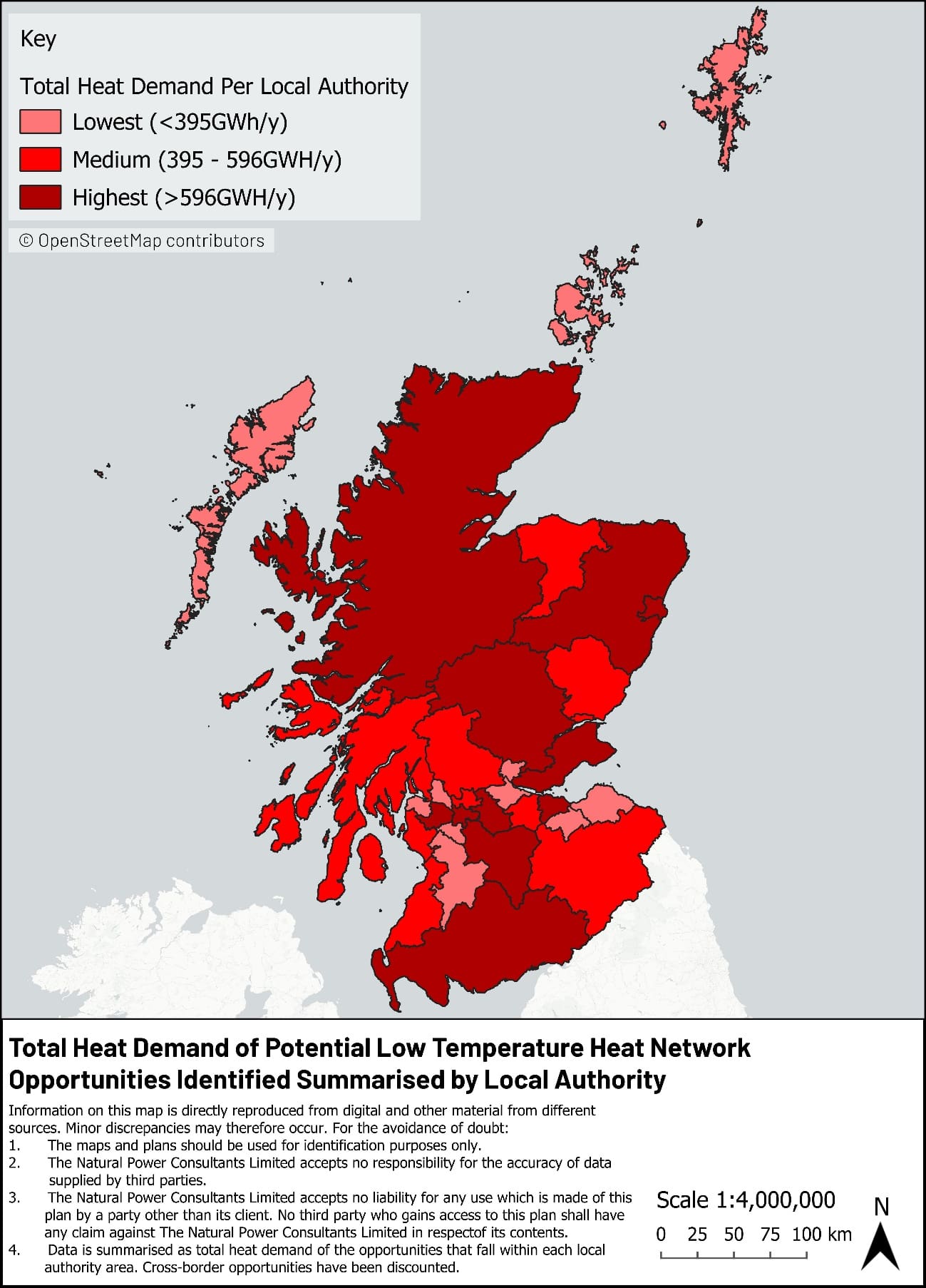
Figure 4: Total heat demand of potential opportunities (Multi-Building Opportunities and Communal Opportunities combined) within local authority boundaries

Table 3 reports the number of opportunities of each type by the local authority within which they are located. Low temperature heat network opportunities can be found in each of Scotland’s 32 local authority areas. The more sparsely populated areas like the Orkney Islands, Shetland Islands and Comhairle nan Eilean Siar (Western Isles) still contain more than 50 opportunities each. The larger cities each contain several thousand opportunity groupings. The map in Figure 3 illustrates the geographic spread of the opportunities identified.

Table 4 presents the total heat demand of each type of opportunity in each local authority area. This data confirms that, while the greatest potential in terms of total heat demand can be found in the larger cities, there is potential for supplying very significant amounts of heat through low temperature heat networks elsewhere in the country. Highland, Fife and Aberdeenshire stand out as areas with large quantities of heat demand contained within Multi-Building Opportunities. Figure 4 presents the total heat demand within both types of opportunity by local authority, using colour coding to differentiate between the areas with the lowest, medium and highest totals.

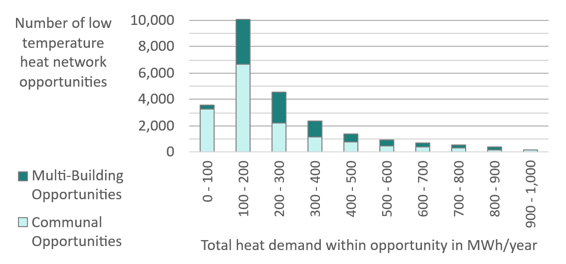
Figure 5: Number of potential low temperature heat network opportunities, by scale of total heat demand within opportunity (within the range 0 – 1,000 MWh per year)

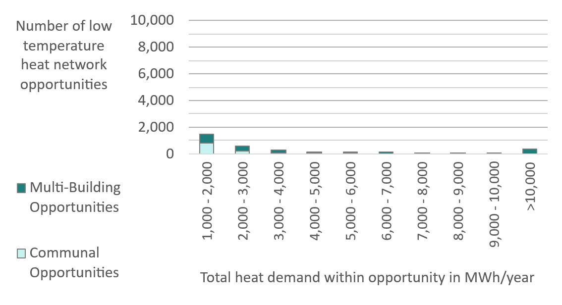
Figure 6: Number of potential low temperature heat network opportunities, by scale of total heat demand within opportunity (within the range 1,000 – 10,000+ MWh per year)

Figure 5 and Figure 6 show the distribution of the low temperature heat network opportunities by scale, grouping opportunities according to their total heat demand. Around a third of opportunities (around 10,000) have a total heat demand between 100 and 200 MWh per year each. This is roughly equivalent to the total heat demand of 10-20 typical 3-bedroom homes.

The majority (89%) of opportunities contain fewer than 100 dwellings and fewer than 10 non-domestic properties. These represent 38% of the heat demand of all opportunities combined.

The proportion containing fewer than 100 dwellings and fewer than 10 non-domestic properties is very similar for both Communal Opportunities and Multi-Building Opportunities (90% and 87% respectively). More than half contain less than 20 dwellings.

Table 5 presents the total number of properties located within each type of opportunity in each local authority area. It confirms that Glasgow and Edinburgh contain the greatest numbers of properties included within both types of opportunity combined (but dominated by Communal Opportunities). Highland and Fife have the largest number of properties contained within Multi-Building Opportunities.

Table 5: Total number of properties within opportunities by local authority

High Property Count Areas and High Heat Demand Areas

High Property Count Areas (HPCAs) were found in all of Scotland’s 32 local authority areas. There are HPCAs in every ‘Large Urban Area’ (areas with more than 125,000 population^[2]) and the majority of ‘Other Urban Areas’ (areas with 10,000 to 124,999 population). Some ‘Accessible Small Towns’ also have HPCAs.

The HCPAs with heat demands exceeding 100,000 MWh per year are also High Heat Demand Areas. Table 6 reports the number and characteristics of the High Property Count Areas and High Heat Demand Areas (the High Heat Demand Area results being a subset of the High Property Count Area results).

Table 6: High Property Count Areas and High Heat Demand Areas results

Figure 7 shows the distribution of HPCAs according to their total annual heat demand.

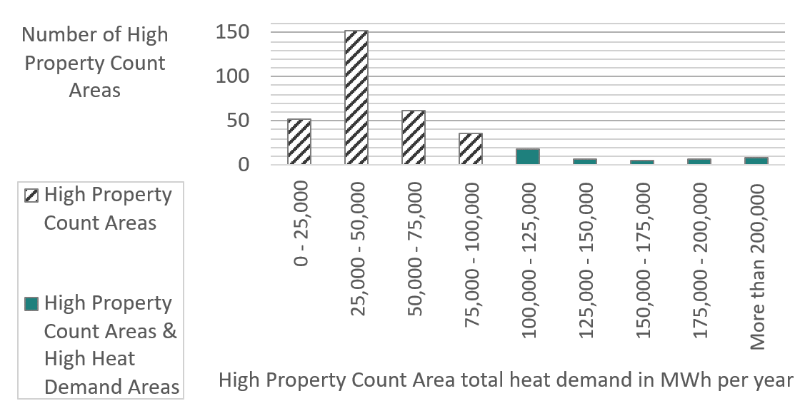
Figure 7: Number of High Property Count and High Heat Demand Areas, by total heat demand

Low temperature heat network archetypes

Table 7 summarises the results of the national assessment, broken down according to the low temperature heat networks defined in Section 4.4.2. There is significant overlap between the groups belonging to each Multi-Building Opportunity archetype, which means that the disaggregated figures do not sum to the totals that apply to their parent category. This is because it is common for more than one archetype to apply to a Multi-Building Opportunity.

It can be seen that a little over a fifth of Multi-Building Opportunities include one or more anchor loads. Half of these include public sector anchor loads, while three-quarters include non-public sector anchor loads. The Anchor Load-Led archetype was not applicable to Communal Opportunities.

More than 85% of opportunities were matched with one or more nearby green spaces. 22,348 (80%) of opportunities had been matched with between 1 and 5 green spaces. A few were matched with a large number of green spaces, with two instances featuring 74 and 96 green spaces matches representing the extremes. In the locations with large numbers of matches, many of the green spaces involved had relatively small areas (although still larger than 1,000 square metres). They included areas of roadside grass, open areas within industrial estates and around public buildings, and patches of uncultivated grassland or scrubland. The number of green space matches is a guide to the diversity of possible places where ground heat collection infrastructure could be located. However, it is not indicative of the total heat generation potential associated with green space within or close to a low temperature heat network opportunity.

Overall, 3,668 opportunities (13%) were matched with one or more blue spaces. Most of these were matched with 1, 2 or 3 water bodies. A small number (52) of opportunities were matched with between 4 and 10 water bodies.

In total, 132 opportunities were matched with waste heat sources, with the majority of these being matched with one nearby site where waste heat is expected to be available. Most of these matched waste heat sources have estimated supply capacities of up to 1,000 MWh per year. However, a minority of the matched sources are estimated to be able to supply up to 10,000 MWh per year, and a few in excess of 30,000 MWh per year.

Table 7: Summary of national results broken down by archetypes

Characteristics of properties within opportunities

Socially rented properties can represent good opportunities for low temperature heat network development thanks to the prevalence of concentrated ownership by organisations with strong incentives to decarbonise their stock. Across the opportunities identified in the model, 40% contain no socially rented dwellings. Among those that do, Communal Opportunities are more likely to include socially rented homes, and for the proportion of homes that are socially rented to be higher. The socially rented proportion averages 36% of dwellings within Communal Opportunities, compared to 16% within Multi-Building Opportunities. 10% of Communal Opportunities (1,557) were found to be wholly socially rented compared to 1% of Multi-Building Opportunities (133).

Fuel poverty is a social dimension that is important to many organisations involved in energy planning and the development of low temperature heat networks. Estimates of the likelihood of domestic properties’ occupants experiencing fuel poverty are available in the Home Analytics dataset. However, the bases of these estimates are not nationally consistent. To reduce the impact of local variability, the datasets generated by the national assessment express fuel poverty prevalence in terms of Lower, Middle and Higher bands rather than quantitatively. These bands were designed to contain roughly equal numbers of low temperature heat network opportunities, such that the Lower band contains the third of opportunities that have the lowest overall fuel poverty prevalence (and so on).

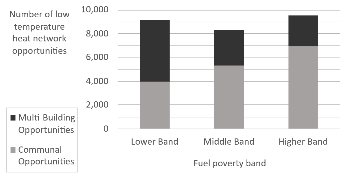
Figure 8: Number of potential low temperature heat network opportunities within each fuel poverty band defined by the national assessment

Figure 8 shows the distribution of opportunities across the fuel poverty bands. The Lower, Middle and Higher bands account for around 303,000, 308,000 and 288,000 dwellings respectively. The relatively even distribution of dwellings across the three bands is a result of their definition: the Lower, Middle and Higher bands refer to the expected average rates of fuel poverty relative to all low temperature heat network opportunities. The bands allow those opportunities with the highest or lowest expected prevalence of fuel poverty to be identified. However, more granular fuel poverty data (such as that available through the Home Analytics dataset) is required to understand the probability of fuel poverty affecting dwellings within an opportunity grouping.

It is notable that Multi-Building Opportunities are over-represented in the Lower band (e.g. these opportunities tend to involve groupings with lower overall prevalence of fuel poverty). The estimated average fuel poverty prevalence within Communal Opportunities is more likely to place them in the Higher band (higher overall prevalence of fuel poverty). This finding conforms to expectations, given that many social homes (often occupied by people with low incomes) are located in blocks of flats.

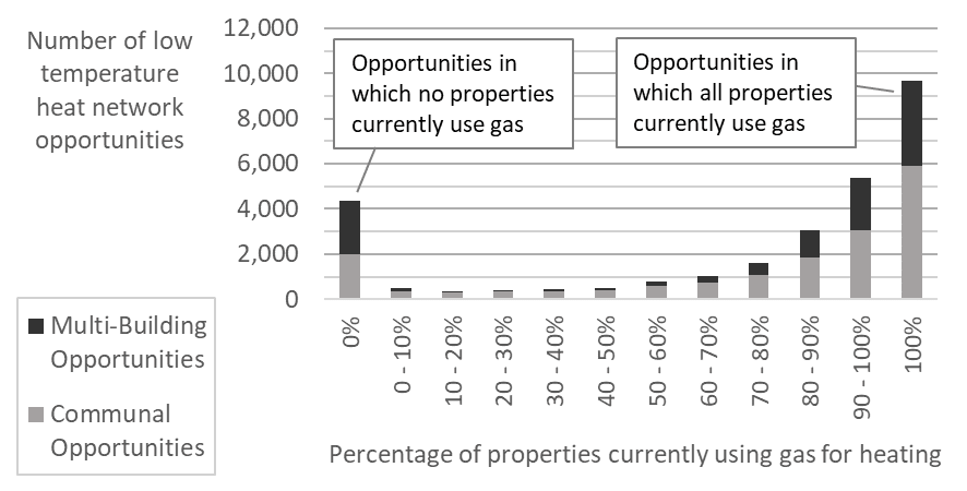
Figure 9: Number of potential low temperature heat network opportunities, by the proportion of properties estimated to currently use gas for heating

Figure 9 illustrates the distribution of the identified opportunities according to the percentage of properties within them that are estimated to currently use mains gas for heating. Well over half of the opportunity groupings are dominated by gas as a heating fuel. However, a notable proportion comprises groups in which no properties use mains gas. Many of these are Multi-Building Opportunities in areas where there is no mains gas grid, or Communal Opportunities in blocks of flats that are electrically heated.

1,724 opportunities (1,461 Communal Opportunities and 263 Multi-Building Opportunities) consist of groupings in which 100% of properties are electrically heated. Electrically heated homes with high heat demands are of particular relevance to fuel poverty, since these homes tend to experience the highest heating costs (or to be underheated in response to high heating costs).

Potential uses of the results

The data outputs produced by the research can be used for purposes that include local and national energy planning, project identification and prioritisation, public engagement (including awareness-raising), business planning and strategy development, knowledge-building and as an input to future research.

Figure 10 depicts the typical development process for a low temperature heat network project, including some of the stages that may be undertaken. The process contains the same activities as are typically undertaken for high temperature heat network projects. This national assessment falls into the very first stage in the process, which is one of strategy development, mapping and masterplanning. Multiple options remain under consideration at this point, including different types, scales and configurations of heat network as well as other low-carbon heat technologies.

The process depicted in Figure 10 is not prescriptive. It is frequently the case – especially for smaller and simpler low temperature heat network projects – that many of the activities and stages shown in the diagram can be undertaken at low cost and with a light touch. Decision-making by private sector heat network developers or property owners engaged in decarbonising their stock might make reference to energy strategies and plans developed by others, and might combine feasibility work with business case development. Multiple stages of design may not be required for lower risk schemes.

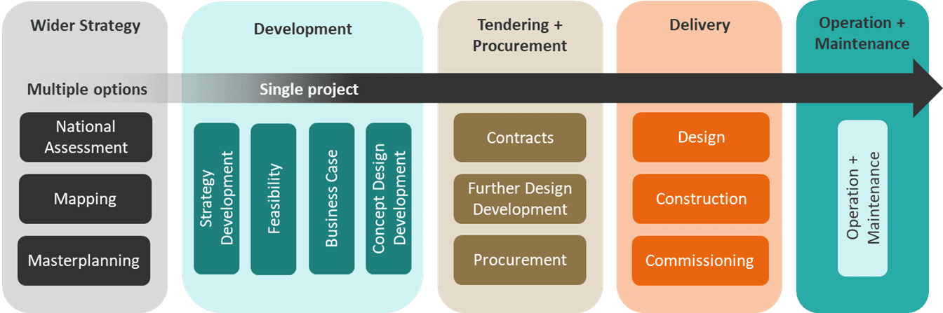
Figure 10: Low temperature heat network project development process (adapted from Heat Network Support Unit materials)

The high-level statistics and charts presented in the previous section could be used to raise the profile of low temperature heat networks as building decarbonisation technology option, and therefore as a means to achieve the objectives of LHEES and national-scale targets. The information presented about opportunity characteristics only scratches the surface of the data that is available regarding each individual opportunity or the aggregated opportunities in an area. Users of the detailed data outputs can use this information to select priority opportunities for further development work. The detailed data may also serve as an input to energy planning processes that consider multiple technologies and energy vectors and the relationships between them. For some organisations, access to the datasets will require signing of and compliance with a data sharing agreement.

Data on the favourability of specific areas for shallow geothermal heat (closed loop and open loop boreholes) will be important for the further assessment of low temperature heat network opportunities in locations where other heat sources are not available. The British Geological Survey’s UK Geothermal Platform is a freely available web-based data resource that could be used to understand the potential yield from underground boreholes in the vicinity of an opportunity.

Characteristics generated by the national assessment that could be used to prioritise places for low temperature heat network development include (among many others):

• The density of opportunities of any type, or of a particular type, could inform supply chain participants’ strategies with respect to geographic focus or types of environments that offer growth potential.
• Social deprivation and fuel poverty probability indicators could enable the identification of places where low temperature heat networks might be able to have a positive impact on fuel poverty.
• Opportunities with a high proportion of socially rented dwellings may represent favourable locations due to the likely concentration of property ownership among organisations with strong drivers to decarbonise heating systems.
• The prevalence of polluting heating systems could enable prioritisation based on potential carbon savings.

Priorities for further work

The following list identifies priorities for further work that have been informed by desk research undertaken in support of the national assessment; stakeholder engagement; and analysis of the limitations of the national assessment methodology. More detailed potential improvements are explored in Section 7 of Appendix A.

• Develop improved evidence regarding the relationship between properties’ heat demands and the maximum distances over which it is viable for them to connect to a low temperature heat network. Conduct sensitivity analysis on the assumptions that the national assessment used to understand the impact on the number and scale of opportunities identified.
• Incorporate more recently-updated heat demand and opportunity characterisation data.
• Expand and update the list of waste heat sources from which potential matches with low temperature heat networks are assessed. In particular, a larger number of wastewater treatment plants as well as recently-constructed and planned data centres could be added along with estimates of their heat supply potential.
• Develop methodologies to analyse the likelihood of construction or relative attractiveness of specific opportunities.
• Improve the evidence base around key topics identified by stakeholders:
  • The cost and affordability of heat from low temperature heat networks, and how it compares to alternatives (including business as usual);
  • Delivery vehicles appropriate to the development of low temperature heat networks;
  • Impacts on and interactions with nearby high temperature heat networks (both operational and planned);
  • Risks associated with the development of low temperature heat networks that differ from other heat infrastructure projects;
  • Timescales applicable to the project development process for low temperature heat networks;
  • Advantages offered by low temperature heat networks (relative to the alternatives) in specific geographical, built environment and social contexts.

Conclusions

Our work provides the first national-scale assessment of locations where there is strong potential for supplying heat through networks that are designed to operate at low temperatures (typically less than 35 degrees centigrade). The results of our assessment can be used for purposes that include local and national energy planning, project identification and prioritisation, public engagement (including awareness-raising), business planning and strategy development, knowledge-building and as an input to future research.

Our approach builds on those previously used in the assessment of high temperature heat network opportunities at national scale, and more localised work focusing on low temperature networks. Future assessments will be able to repeat and/or build on a tested, refined and documented methodology that has been designed with replicability in mind.

Our national assessment identified a total of 11,109 Multi-Building Opportunities and 16,985 Communal Opportunities across Scotland. These opportunity groupings collectively represent around 900,000 dwellings and 100,000 non-domestic properties. They include around a third of the country’s housing stock and around a third of Scotland’s non-domestic properties. In practice, not all properties within the identified opportunities are likely to choose to or be able to connect to a network. These totals represent an estimate of the potential, given the assumptions made and within the range delineated by the identification and classification criteria used (minimum and maximum property counts).

The majority of the opportunities identified involve relatively small numbers of heat-using properties. However, there are also a small number of opportunities with high significance in terms of their total heat demand. These include groupings with a large number of properties and those with one or more large anchor loads. Around 350 opportunities have total heat demands exceeding 10,000 MWh per year. High Property Count Areas represent a further approximately 350 groupings with total heat demands ranging from around 13,000 MWh to around 290,000 MWh.

The findings also support the idea that the future market for low temperature heat networks could potentially be much larger than it is at present. That said, this research has not compared low temperature heat networks against other zero-emissions heating solutions or sought to identify optimum solutions. The actual contribution that low temperature heat networks can make to net zero will depend on the number and characteristics of places in which they represent the ‘best’ solution. Small- and medium-scale high temperature networks may be more cost effective than low temperature heat networks in some of the contexts drawn out by this research.

Low temperature heat network opportunities can be found in each of Scotland’s 32 local authority areas. When depicted on a map, the concentrations of opportunities in the country’s more heavily populated regions (the Central Belt and the urban areas around Aberdeen and Dundee) are evident. However, it is also clear that opportunities can be found in the majority of Scotland’s towns, and in rural and coastal villages throughout the Scottish mainland and islands. Opportunities exist right up to the country’s extremities: from Unst to the Rhins of Galloway, and from Barra to the Berwickshire coast. This finding supports the conclusion that all Scottish local authorities should consider low temperature heat networks in future iterations of their LHEES. It could also support decision-making in the supply chain by organisations that may be planning entry into new geographic markets. Other possible uses of the findings regarding geographic distribution relate to electricity infrastructure planning and regional economic development activities.

The information generated about individual opportunities allows them to be ranked and prioritised relative to other opportunities, supporting project identification. This could be relevant for owners of property portfolios (including Registered Social Landlords) as well as heat network project developers. However, the data outputs associated with any one opportunity must be viewed as indicative, and suitable for justifying further project development work rather than supporting significant project-level decisions.

In conclusion, the national assessment provides important new information concerning the potential for supplying heat through low temperature heat networks in Scotland. Provided that the limitations associated with its ‘first pass’, top-down and experimental nature are appropriately recognised, the national assessment can immediately and meaningfully support energy planning initiatives and project identification. The approach developed is suitable for future replication, giving it the potential to contribute to the reduction of greenhouse gas emissions in the built environment over a longer timescale. It provides a national evidence base to support further investigation and informed decision making on low temperature heat networks.

References

AECOM, 2025. Optimising Data Centres in London – Heat Reuse (for Greater London Authority). Available at: https://www.london.gov.uk/sites/default/files/2025-06/Optimising_Data_Centres_in_London_-_Heat_Reuse_250605.pdf (Accessed: 05 January 2026).

Argyll and Bute Council, 2024. Local Heat and Energy Efficiency Strategy (version from Council meeting pack dated 21 November 2024).

Averfalk H et al., 2021. Low-Temperature District Heating Implementation Guidebook: IEA DHC Report. Available at: https://www.iea-dhc.org/fileadmin/documents/Annex_TS2/IEA_DHC_Annex_TS2_Transition_to_low_temperature_DH.pdf (Accessed: 02 February 2026).

Barns et al., 2026. Opportunities and costs for shared ground loops. Renewable and Sustainable Energy Reviews, 228, 116490. Available at: https://doi.org/10.1016/j.rser.2025.116490.

Brummer and Bongers, 2019. Mijnwater Heerlen: Roadmap to 2040. Available at: https://vb.nweurope.eu/media/10451/heatnetnwe_heerlen-transition-roadmap_district-heating.pdf (Accessed: 02 February 2026).

CIBSE, 2008. Energy benchmarks: TM46:2008.

Data Center Map, 2025. Available at: https://www.datacentermap.com/ (Accessed: 16 December 2025).

DESNZ, 2025. UK Geothermal Platform: Summary layers methodology and user guidance. Available at: https://assets.publishing.service.gov.uk/media/68920a0cdc6688ed50878476/uk-geothermal-platform-summary-layers.pdf (Accessed: 21 January 2026).

Element Energy, 2023. Low Carbon Heat Study – Phase 1 (for The Kensa Group). Available from: https://www.erm.com/contentassets/553cd40a6def42b196e32e4d70e149a1/low-carbon-heat-study—phase-1.pdf (Accessed: 04 February 2026).

Energy Saving Trust, 2025a. Home Analytics Scotland v4.0: Release Notes.

Energy Saving Trust, 2025b. Non-Domestic Analytics (NDA) Scotland v2: Release Notes.

Fernández et al., 2025. The integration of heat pumps into the thermal systems of hospital facilities to advance their transformation towards Zero-Emission Buildings. Journal of Building Engineering, 111, 113531. Available at: https://doi.org/10.1016/j.jobe.2025.113531.

Few et al., 2023. The over-prediction of energy use by EPCs in Great Britain: A comparison of EPC-modelled and metered primary energy use intensity. Energy and Buildings, 288, 113024. Available at: https://doi.org/10.1016/j.enbuild.2023.113024.

Greenspace Scotland, 2021. ParkPower Methodology Report: Green Heat in Greenspaces (GHiGs).Available at: https://www.greenspacescotland.org.uk/Handlers/Download.ashx?IDMF=335590f1-e4bb-4dea-b2fd-904fe6b1e3c8 (Accessed: 21 January 2026).

Historic England, 2025. The Viability of Ground Source Heat Pumps in Historic Buildings. Available at: https://historicengland.org.uk/images-books/publications/viability-ground-source-heat-pumps-historic-buildings/heag327-gshp-historic-buildings/ (Accessed: 04 February 2026).

Johnston et al., 2024. The suitability of clean heating options for challenging dwelling types. ClimateXChange. Available at: https://www.climatexchange.org.uk/wp-content/uploads/2024/10/CXC-The-suitability-of-clean-heating-options-for-challenging-dwelling-types-September-2024.pdf (Accessed: 23 December 2025).

Kensa Group Response: Environmental Audit Committee Inquiry Heat resilience and sustainable cooling August 2023. Available at: committees.parliament.uk/writtenevidence/123197/pdf/ (Accessed: 21 January 2026).

Scottish Futures Trust, 2024. Heat Networks Delivery Models: report for the Scottish Government. Available at: https://www.gov.scot/binaries/content/documents/govscot/publications/advice-and-guidance/2024/02/heat-networks-delivery-models/documents/heat-networks-delivery-models-final-report/heat-networks-delivery-models-final-report/govscot%3Adocument/heat-networks-delivery-models-final-report.pdf (Accessed: 04 February 2026).

Scottish Government, 2022. Heat networks delivery plan. Available at: https://www.gov.scot/publications/heat-networks-delivery-plan/ (Accessed: 18 February 2026).

Sinclair and Unkaya (BRE) for ClimateXChange, 2020. Potential sources of waste heat for heat networks in Scotland. Available at: http://dx.doi.org/10.7488/era/730.

South of Scotland Enterprise, 2025. South of Scotland Heat Networks Prospectus. Available at: southofscotlandenterprise.com/media/gaffpjka/final-heat-networks-prospectus-for-the-south-of-scotland-sose-compressed.pdf (Accessed: 22 January 2026).

UK Government, 2025. Analytical Note on Alternative Low Carbon Heating Technology Costs. Available from: https://assets.publishing.service.gov.uk/media/6917213f9d50fc2fe8161800/alternative-low-carbon-heating-technology-costs-analytical-annex.pdf (Accessed: 04 February 2026).

Zero Waste Scotland, 2022a. First National Assessment of Potential Heat Network Zones. Available from: https://www.gov.scot/publications/first-national-assessment-potential-heat-network-zones/documents/ (Accessed 21 February 2026).

Zero Waste Scotland, 2022b. LHEES Stage 4: Generation of initial delivery areas. Heat decarbonisation: Off-gas grid Detailed Practitioner Approach, version 4.0. Available at: cdn.zerowastescotland.org.uk/managed-downloads/mf–mafxpwo-1719911460d (Accessed: 21 January 2026).

Zero Waste Scotland, 2022c. LHEES Stage 4: Generation of initial delivery areas. Heat decarbonisation: On-gas grid Detailed Practitioner Approach, version 4.0. Available at: cdn.zerowastescotland.org.uk/managed-downloads/mf-xirknd2o-1719915354d (Accessed: 21 January 2026).

Zero Waste Scotland, 2024. Identifying opportunities for shared loop GSHP: Principles to indicate specific prospects (Confidential).

Appendices

Introduction

This Appendix begins by setting out the ‘model’ scope and specifications, where the ‘model’ is defined as the process for delivering the national assessment of low temperature heat network opportunities using input datasets, assumptions, calculations and geospatial processes. Chapter 4 of this Appendix sets out the key decisions that shaped the design of the model: the strategic approach; key concepts, assumptions and limitations; screening decisions; and data quality risk assessment and mitigation. Chapter 5 sequentially lists the steps followed to execute the model. The final sections discuss the quality assurance activities carried out by the researchers and Scottish Government representatives, and then go on to discuss potential improvements.

Model scope

Summary statement

The model delivers a national assessment of locations that are potentially suitable for low temperature heat networks in Scotland. The research supports the Scottish Government’s priority to reduce greenhouse gas emissions in the buildings sector.

Model details

Key outputs

The key outputs generated by the model are:

• geospatial polygons representing Multi-Building Opportunities and High Property Count Areas (both defined later in this Appendix), with attribute data;
• geospatial points representing Communal Opportunities, Public Sector Anchor Loads, Other Anchor Loads, Potential Heat Sources and Potential Cooling Customers (all defined later in this Appendix); and
• geospatial data presentations (geopackages) which allow different elements of the polygons/points and their distributions to be viewed and interpreted.

Key inputs

The key data sets used by the model are the Scotland Heat Map 2022, Home Analytics v4.1, Non-Domestic Analytics v2.0, Green Heat in Greenspaces and the UK Geothermal Platform Summary Layers.

Boundaries and geographic scope limitations

The spatial extent of the model is the areas enclosed by (collectively) the boundaries of the 32 Scottish local authority areas, plus (where not already included) water bodies within 100 metres of local authority areas. The built environment modelled is limited to those properties which have demand for heat and feature in the 2022 Scotland Heat Map, which means it does not include recent new build or planned developments.

The low temperature heat network opportunities identified are not influenced by the presence of demand for cooling, which in practice could improve project viability. However, potential larger cooling customers within heat network opportunity groupings have been identified.

Model specifications

For the purposes of this section, the ‘model’ is defined as the process by which the national assessment has been delivered.

The model was required to identify locations likely to be suitable for low temperature heat networks in Scotland, and to generate data outputs that characterise the potential opportunity at each location. From these data outputs, national-level or regional-level numerical summary results were generated.

The model was also required to generate mapping visualisations that users could use to understand the distribution of opportunities across Scotland and at a more localised level, and to inspect individual opportunity locations. Geospatial data outputs were required in order that certain users could incorporate the results of the national assessment into their own geospatial information systems (GIS) environments, integrate with their own data and perform their own follow-on analysis.

The map visualisations and geospatial data outputs also illustrate the distribution of characteristics and conditions that tend to make a location suitable for low temperature heat networks. Users can use these characteristics to carry out their own prioritisation of opportunities.

The model comprises data inputs, calculations and processes and data outputs.

Data inputs

The datasets that provided inputs to the model are listed in Table 8.

Table 8: Data inputs, summary of pre-processing and summary of data quality assessment

An additional dataset has been compiled by the researchers from a web search for operational and planned data centres in Scotland.

User inputs

Users will only interact with the outputs of the model, which represent a single, static scenario. Users viewing the outputs through GIS software will be able to select different pre-defined views of the data, and to apply filters to create their own desired presentations. Users will not specify any parameters that influence the outputs, although they will be able to create modified versions of the outputs (including adding or deleting geospatial features and overwriting attributes). A master copy of the outputs will be held by Scottish Government and represents an unaltered ‘single source of truth’.

Model outputs

Table 9 lists the layers included in the geospatial data outputs.

Table 9: Data outputs

Table 10 lists the visualisations that were created and included in the geopackages for the purpose of assisting users to understand the spatial and statistical distributions of different parameters. Not all visualisations are made available to all users (as per data sharing arrangements).

Table 10: Geospatial visualisations

Calculations and processes

Figure 11 summaries the logical steps that lead to the delivery of the spatial polygons and point data that comprise the model outputs.

Figure 12 summarises the high-level processes that match non-contiguous heat sources to opportunities for the purposes of opportunity characterisation.

Output: Multi-Building Opportunity and High Property Count Area datasets

Output: Communal Opportunity datasets

** The main working dataset is a data-minimised version of the ‘Heat demands’ layer of the Scotland Heat Map, with minor additions created in Step 2.

* The creation of a geospatial layer representing physical barriers was an activity carried out in parallel to Steps 1 to 4.

Figure 11: Flow chart summarising the high-level processes leading to the data outputs

Figure 12: Flow chart summarising the high-level processes that match non-contiguous heat sources to opportunities for the purposes of opportunity characterisation

Software requirements

The geospatial outputs are provided in a format that can be opened by all major Geospatial Information Systems (GIS) software packages.

Model design

The model comprises data inputs, calculations and processes and data outputs. The data inputs and data outputs exist in static format, with their version indicated in filenames and accompanying documentation. The calculations and processes that generated the data outputs are documented in this section and Section 5 of this Appendix but are not otherwise retained. The model does not require maintenance.

An Assumptions Log accompanies the data outputs. All assumptions listed in the Log have been addressed in this Appendix.

Data quality impacts were assessed, and for the most part the response was to accept the impacts as a limitation of the methodology. In this chapter, data accuracy considerations are discussed alongside the concept to which they relate.

The input datasets used represent the most comprehensive datasets available that are fit for the purpose required. However, for a small number of issues, active responses were developed and are described in this chapter and Section 5.1.3.

Strategic approach

The model design aimed to identify clusters of heat demands that correlate reasonably well with real-world opportunities for low temperature heat network deployment, but aimed to minimise the influence of more subjective assumptions. By attaching informative attributes to the groupings, they become characterised opportunities. These attributes highlight those aspects that could significantly influence the attractiveness of the opportunity to certain stakeholders (who will bring their own implicit weightings to the different characteristics). The exception to this is a scale-based screening parameter that has been applied to ensure that outputs are manageable in number (preferring a large number of reasonably-sized opportunities over a very large number of opportunities dominated by very small schemes).

Stakeholder engagement

The development of the methodology for the national assessment was supported by a multi-stage programme of stakeholder engagement involving a broad range of organisations. This engagement ensured that the research approach, underlying assumptions and emerging findings were informed by the practical experience, operational knowledge and strategic priorities of organisations active in Scotland’s heat, energy and infrastructure sectors.

A series of four stakeholder events were delivered during the research period, comprising two workshops in August 2025 and two workshops in November 2025. These events brought together representatives from local authorities, network operators, public bodies, heat network developers, community energy groups, national agencies and academic or technical specialists. All 32 Scottish local authorities were invited to attend these events, ensuring that every council had the opportunity to contribute local knowledge and perspectives. The workshops enabled participants to: 

• review and discuss the emerging methodology for identifying low temperature heat network opportunities; 
• provide feedback on key modelling assumptions, including definitions of opportunity types, thresholds, and data inputs; 
• explore early spatial outputs and identify areas where local knowledge could complement national datasets; 
• highlight known constraints, operational considerations and integration challenges relevant to heat network deployment; and
• share examples of ongoing or planned heat decarbonisation activity that could influence interpretation of the assessment outputs. 

In addition to the group workshops, we held a series of one-to-one meetings with key stakeholders to gather deeper technical insights and address topic-specific considerations. Organisations engaged through these targeted discussions included Scottish Power Energy Networks (SPEN) and the British Geological Survey (BGS). 

Collectively, the stakeholder engagement process strengthened the robustness of the national assessment, helping to validate the suitability of key assumptions, highlight limitations inherent in national scale datasets, and ensure that the final geospatial outputs are aligned with the needs and expectations of future users—including local authorities, public sector organisations and industry partners. 

Model concepts, assumptions and limitations

Heat demands and distances between potential connections

Heat demand proximity analysis assumptions

The amount of heat needed by an individual property has a very strong influence on the distance over which it is viable to connect its heating system to a local heat network. The national assessment took an approach common to most other relevant past assessments: calculating an estimated maximum connection distance between heat demands that was directly proportional to the sum of the heat demands.

For almost all properties, the formula used to calculate the maximum connection distance was:

The divisor of 2,000 (units: kWh per year per metre) is a proxy for the Linear Heat Density that could be achieved by the relevant section of a low temperature heat network. The Linear Heat Density (LHD) is a measure of the amount of heat supplied through part or all of a heat network relative to the total length of pipe route in that (part-)network. For prospective heat network opportunities, the LHD is a relatively strong indicator of the likely financial viability of the network. A high LHD implies that more heat will be supplied (generating revenue and/or cost savings) through a shorter amount of pipework (costing less to install and maintain).

Stakeholders were consulted on the fundamentally influential LHD-proxy assumption of 2,000 kWh per year per metre, with general support expressed for this value. It also aligns with a value used in a previous assessment carried out by Zero Waste Scotland and Buro Happold for low temperature heat networks in Argyll and Bute, which was informed by engagement with an experienced low temperature heat network developer. This assumption was further justified through our development of prototype comparative cost models.

The Linear Heat Density of a theoretical pipe route that connects two individual buildings is conceptually different from the overall Linear Heat Density of a heat network. The latter measure takes into account the fact that pipe routes often deviate significantly from the shortest possible route between two points, and that not all buildings within a defined area will necessarily have connected to the network. The overall LHD of planned and operational low temperature heat networks can be less than 2,000 kWh per year per metre, often considerably so. Averfalk et al. for IEA (2021) assessed 37 heat networks across the world, most of them low temperature heat networks or operating at less than 65 degrees centigrade for most of the year. The authors found that almost half of these networks exhibited values below 1,000 kWh per year per metre including delivered cooling energy as well as heat (meaning that their heat-only LHD could be even lower).

It is possible that schemes exhibiting lower heat demand densities can be viable. A major developer of low temperature heat networks suggested in a submission to the UK Parliament Environmental Audit Committee (Kensa, 2023) that a heat demand density of 500 kWh per metre per year could indicate viability. However, the aim of this research to identify locations likely to be suitable for these types of heat networks (rather than only possibly suitable) justifies the selection of a higher number.

If the LHD-proxy value chosen had been higher, fewer opportunities would have been identified, and they would have tended to be smaller. If the LHD-proxy value had been lower, more opportunities would have been identified, and they would have tended to be larger.

It is recommended that any future studies that require an LHD-proxy value for the identification of low temperature heat network opportunities assess the evidence available at the time to select an appropriate assumption.

There is on average a difference between real-world heat consumption of a property (lower) and the estimated heat demand in the dataset used (higher) (Few et al., 2023, and discussed in more detail in Section 4.2.1.3). The selection of a 2,000 kWh per metre per year divisor, rather than a lower figure, offers the benefit of slightly compensating for the overestimation of heat consumption.

One group of properties for which a different divisor was used was public sector anchor loads. In recognition of the strong motivations that the owners of these properties have to decarbonise (among other factors), a divisor of 1,500 kWh per metre per year was used. This assumption was also tested and agreed with stakeholders.

When identifying spatially dispersed Multi-Building Opportunities, we applied a limit of 1 km to the maximum distance over which two buildings can be grouped into an opportunity (without there being additional buildings in between). This meant that the distance between buildings within an opportunity area did not risk being unrealistically large. However, in exceptional circumstances, connections exceeding the 1 km threshold adopted could be feasible. For example, a building with a very large heat demand, such as a hospital or higher education campus, may be separated from other buildings by open space through which it is reasonably cheap to construct a pipeline. The viability of a heat network involving this long connection could be further enhanced if an attractive heat source could be accessed by connecting across the space; if the land between is under single ownership or a small number of owners; or if the large heat user exhibited low seasonality in its heating demand or required cooling outside the heating season.

If the maximum connection distance had been higher, more opportunities would have been identified, and they would have tended to be larger (and vice versa).

Heat demand proximity analysis mechanics

An important distinction between two types of low temperature heat network concerns the number of buildings which are served by the network. Our process separated ‘Communal Opportunities’ (blocks of flats, tall tenement buildings and large multi-occupancy commercial buildings) from opportunities that consist of clusters of separate buildings. Communal Opportunities were identified by grouping heat demands that shared a building footprint in the Ordnance Survey MasterMap Buildings data layer, and where the majority of heat demand records infer that the estimated building height is at least 7.5 metres. Although not perfect, these criteria tend to include blocks of flats, tenements and taller mixed-use buildings while excluding houses.

Buildings whose height has been overestimated will have occasionally been misclassified as a Communal Opportunity. However, this categorisation is arbitrary – and despite the building’s height it is still possible that a communal system is appropriate. If a building’s height has been underestimated, a genuine opportunity for a communal system may have been missed – but the heat demands in that building will have had the chance to be picked up in a Multi-Building Opportunity.

Once the heat demands that had been grouped into Communal Opportunities had been identified, the master dataset of heat demands was separated into two parts: one containing the heat demands belonging to Communal Opportunities and one containing all other heat demands. The latter part-dataset went forward to the Multi-Building Opportunity identification process.

The Communal Opportunities did not form part of the Multi-Building Opportunity identification process. The approach taken ensures that Communal Opportunities are not double counted when low temperature heat network opportunities are considered as a whole. Communal Opportunities often represent locations where real schemes could be implemented relatively simply and potentially quickly.

A potential limitation of this approach is that some buildings near to Communal Opportunities, but which are not close enough to other individual or smaller multi-property buildings, may not be identified as belonging to any low temperature heat network opportunities. Rarely, a Communal Opportunity might form a ‘bridge’ between two small clusters of buildings that on their own fall short of being identified as Multi-Building Opportunities. These limitations are expected to have a relatively small impact on the overall results of the national assessment. If a particular Communal Opportunity is subject to further project development investigation, the potential to extend the network to nearby buildings should be considered. Similarly, the potential for the properties in the building to be served from a wider multi-building network (perhaps centred on an anchor load or accessing attractive heat sources) should be considered.

To identify sets of buildings that could be grouped together into Multi-Building Opportunities, spatial buffers were created around the point locations of heat demands. The radius of these circular buffers was calculated for each point using the estimated heat demand and the LHD-proxy values, enforcing the 1km maximum radius described in the previous section. Where the buffer circles overlap, heat demands have the potential to be linked to each other in a single grouping. If no overlap occurs, heat demands cannot be part of the same cluster. Various additional steps, described in subsequent sections, deal with the influence of physical barriers and inclusion/exclusion criteria for the groups that are generated.

The proposed proximity analysis methodology was explained to stakeholders in advance of its final selection and execution. Stakeholders expressed agreement with the suitability of this approach to the purpose of identifying low temperature heat network opportunities.

Heat demand accuracy

Other than its location relative to others, the estimated heat demand of a particular address is the main parameter that determines whether it is included in an opportunity grouping or not. The total heat demand of an opportunity group is also an important piece of characterising information. The dataset from which heat demand estimates were taken is the Scotland Heat Map 2022 (SHM). The vast majority of the heat demand estimates in the dataset used are modelled values rather than measured values.

Consideration was given to using the more recent heat demand estimates available in the Home Analytics and Non-Domestic Analytics datasets. However, it was determined that the advantages offered by the newer datasets were offset by the risk that errors would arise in the matching and merging processes that would be required to integrate datasets that each represent snapshots at different points in time. For example, the classification of residential institutions has changed in recent years.

The SHM heat demand estimates are derived from multiple sources. The highest-confidence values are collected from energy billing or procurement data or derived from metered energy consumption. Medium-confidence estimates are derived from Energy Performance Certificates (the production of which involves physical surveys and some building energy modelling) or Home Analytics modelling.

The lowest-confidence estimates derive from floor area, building age and property type or building use information (with some of these parameters inferred by modelling if they are not known^[4]). The low-confidence estimates rely on benchmark heat demand figures according to building use (non-domestic properties) or property age and type (dwellings). The benchmarks are subject to adjustment where insulation is present, or to account for climatic variation across Scotland. Full detail on the derivation of heat demand estimates can be found in the Scotland Heat Map User Guide (Scottish Government, 2023).

The Home Analytics modelling that underlies almost half of domestic heat demand estimates in the SHM is generally representative of the Scottish housing stock. It is reasonably accurate in terms of its ability to replicate the heat demand estimates generated by the Energy Performance Certificate (EPC) production process (Energy Saving Trust, 2025a). However, the production of EPCs itself involves some simple modelling of a property’s heat requirements based on observations made during a physical survey. EPCs – and therefore any modelling that tries to achieve good correlation with EPC heat demand estimates – tend to overestimate heat demand relative to real-world consumption (Few et al., 2023). If heat demand estimates were more realistic (generally lower), fewer opportunities would have been identified through the national assessment, and they would have tended to be smaller.

The version of the Scotland Heat Map used for the national assessment did not incorporate heat demand estimates from the Non-Domestic Analytics dataset. Instead, heat demands are either estimated from building use classifications, floor areas and benchmarks; from EPCs; or from energy billing data collected from various public sector organisations. For non-domestic properties, the heat demands estimated using benchmarks (least confidence) vastly outnumber those derived from EPCs, which in turn outnumber those derived from billing data (best confidence). Furthermore, the heterogeneity of non-domestic properties further reduces the confidence that can be placed in modelled heat demand estimates, whether they were produced for the purposes of an EPC or calculated using benchmarks (Energy Saving Trust, 2025b).

For the national assessment, the impact of uncertainty in non-domestic heat demand estimates is likely to be greater than the impact of uncertainty in domestic heat demand estimates. This is because almost all of Scotland’s larger “anchor load” heat demands are non-domestic, and non-domestic heat demands are on average higher than domestic heat demands. These facts, combined with the level of uncertainty that applies to non-domestic heat demands, impact the results of the national assessment in the following ways:

• Non-domestic properties’ proportionally larger contribution to opportunity groupings’ heat demand translates into amplified uncertainty on the total heat demand of an opportunity grouping that includes non-domestic properties (and any quantities or conditions derived from the heat demand, including the matching of heat sources to opportunity groupings).
• Non-domestic properties tend to be possible to connect to other buildings over larger distances. These distances can be considerable (up to 1km). In proximity analysis, ‘anchor loads’ often enable the inclusion of many smaller heat demands that fall within their maximum connection radius. Overestimated anchor load heat demands will tend to result in anchor load-led opportunities that are larger in area, have higher property counts and have higher total heat demand than would otherwise be the case. Underestimated anchor load heat demands will have the inverse impact, with the additional result that in some instances opportunity groupings may be missed entirely if they fall below the property count thresholds chosen for the national assessment.

The SHM and Home Analytics datasets are unavoidably biased towards newer, urban properties that have recently been built, bought, sold or had significant retrofit work completed (thus triggering the requirement for an EPC to be produced and lodged). This means that, in general, there is lower confidence in the data reported for rural areas.

Heat demand outliers, unfeasible heat demands and distance constraints

The national assessment dealt with exceptionally large heat demands both through the imposition of limits within heat demand proximity analysis and through selected overwriting of heat demand data.

The maximum distance between potential connections was not allowed to exceed 1 km. This action reflects real-world constraints that are likely to apply, but also effectively places a cap on the influence of an individual property’s heat demand in terms of the formation of a cluster, thereby nullifying large outliers.

In general, as the distance in between two heat demands increases, the probability of encountering one or more obstacles that are very difficult or expensive to cross increases. The cost and/or difficulty of passing such obstacles may not be justified, rendering the connection unviable. Longer distances also tend to incur greater pumping costs and, where applicable, greater heat losses. It is therefore appropriate to set a threshold distance above which it is assumed that the likelihood of a connection being viable becomes low. One of the world’s largest low temperature heat networks in Heerlen, Netherlands, involves maximum inter-building distances of 800 to 1,000 metres as the crow flies (Brummer and Bongers, 2019).

The Scotland Heat Map contains a small number of erroneous outlier heat demands. We concluded that around 16 of the 41 largest heat demands (those estimated in the SHM to consume more than 20,000 MWh per year) were overestimated by a factor of 10 or more, based on consideration of the floor area and the most energy-intensive heat demand benchmark from CIBSE’s TM46 Energy Benchmarks publication (CIBSE, 2008). These 16 heat demands represent less than 0.01% of the non-domestic heat demands in the SHM, and less than 0.001% of all heat demands in the SHM. A further 12 of the largest heat demands were also determined to be likely to have been overestimated, but to a smaller degree.

These 28 outlier heat demands were edited for the purposes of calculating the total heat demand within an opportunity grouping, to improve the accuracy of opportunity characteristics and the statistics derived from them. This adjustment reduced the number and impact of unrealistic totals reported as characteristics of opportunities. Adjustments were only made to non-domestic properties with a heat demand exceeding 20,000 MWh per year, and a reported ‘confidence level’ which suggested that the heat demand had been modelled rather than being based on actual reported energy use. The heat demand was reduced to 20,000 MWh/year or 1 MWh/m²/year (whichever was lower). This does not represent a theoretical maximum demand that can be connected to a low temperature heat network, but rather an adjustment to reduce the impact of very large potentially erroneous heat demands.

Considering buildings that are typically space heated throughout (i.e. excluding industrial sites and distribution and logistics centres), many of Scotland’s largest properties by floor area are hospitals and higher education buildings. These large public buildings often have heat demand estimates that are derived from metered consumption data (hence have a high confidence level). Consideration of the metered heat demand figures for Scotland’s largest hospitals and higher education buildings leads to the conclusion that the country’s largest combined space heating and hot water loads are in the region of 20,000 MWh per year (only one hospital exceeds this value). The overwriting process described in the previous paragraph does not impact the heat demand estimates for hospitals or higher education facilities where their ‘confidence level’ is the highest value (5).

The second criterion for limiting heat demand estimates is justified by consideration of fuel demand benchmarks included in CIBSE’s TM46 Energy Benchmarks publication (CIBSE, 2008). Of the 29 categories of building for which energy benchmarks are stated, the most heat-intensive is “Swimming pool centre”, with a benchmark of 1,130 kWh per year per square metre of floor area. This benchmark is stated in terms of fossil fuels used for heating, meaning that it corresponds approximately to a heat demand of 1,000 kWh (or 1 MWh) per year per square metre. The researchers chose to use this value as representing the highest reasonable heat use intensity for the purposes of adjusting large outlier heat demands.

These 28 heat demand adjustments result in a reduction of between around 1,000 MWh/year (smallest adjustment) and 1,000,000 MWh/year (largest adjustment) in the heat demand of the opportunity groupings in which these properties lie. These adjustments affect the total heat demand of relevant opportunity groupings, but not the list of properties included in the groupings (because maximum connection distances were already capped at 1km, meaning that all heat demands above 2,000 MWh/year (or 1,500 MWh/year for public anchor loads) have the same maximum connection distance).

A further adjustment was made to hospitals with heat demands exceeding 10,000 MWh per year, regardless of the basis of the heat demand value. This adjustment sought to account for the fact that in medium-to-large-sized hospitals a significant proportion of the overall heat demand relates to uses that can be served only from high-temperature sources. An energy model of a medium-sized hospital in Spain was developed by Fernández et al. (2025). The researchers went expanded the simulation to additional locations, including London. The London results were used to estimate the proportion of heat demand that could be met from a low temperature heat network supplying heat into existing hot water distribution systems. (The heat demanded by existing steam-using systems was assumed to be not easily met from a low temperature heat network. Multi-stage steam-generating heat pump systems are technically feasible but offer minimal operational cost benefits relative to electric steam generators, which are cheaper to install.) The assumed proportion of hospital heat demand that was included in aggregated heat demand totals within opportunity groupings was 42.5%. An adjustment was applied to a total of 17 hospitals.

It was noted through work on this assessment, and our past experience working with the Scotland Heat Map, that one circumstance that can lead to outlier heat demands is a large supermarket with one or more concessions within it and/or an internal café restaurant. Anomalous heat demands occur when the large floor area of the supermarket is divided equally between several use classes (as per the methodology followed in the development of the SHM), rather than the actual floor areas being applied. The heat demand benchmark for the “Restaurant / Cafeteria” use class is more than 3 times higher than the benchmark for the “General Retail” use class. A high heat demand benchmark therefore gets applied to a falsely large floor area that has been assigned the “Restaurant / Cafeteria” use class.

The prevalence of this circumstance within West Lothian and an area of Glasgow peripheral to the city centre was investigated. While several instances were noted of “Restaurant / Cafeteria” UPRNs having high assigned floor areas, some of these shared a building with other heat-intensive use classes (e.g. Hotel). It was therefore decided that adjusting “Restaurant / Cafeteria” heat demands across the board was not appropriate.

Influence of physical barriers

The aim of the national assessment was to identify locations likely to be suitable for low temperature heat networks in Scotland. This meant that the identification process needed to take constraints into account, including physical barriers to construction.

Ordnance Survey mapping layers (from the OS Zoomstack product) were used to create a combined “Barriers” spatial dataset. This was then used to cut the heat demand buffer areas, effectively representing some of the physical features that often prove too costly or impossible for low temperature heat networks to cross. The barriers applied include major roadways (motorways and A-roads), railways, woodlands and waterways.

The application of these barriers in the analysis of spatially dispersed heat demand groupings had a direct impact on opportunity identification, preventing connectivity across features that pose a high likelihood of obstructing or increasing cost and complexity for a heat network. The resultant opportunities are therefore smaller, more realistic zones of demand.

However, the mapping of the physical features did not entirely meet the needs of this assessment. Sometimes gaps in the mapped ‘barrier’ features (such as bridges over watercourses) prevent clusters from being cut fully. This means that they remain as a single polygon and are treated as a single Multi-Building Opportunity. Consequently, a barrier with a gap in the wrong place does not have an impact on the final clusters. This is reasonable in the case where a real physical feature like a bridge happens to provide an opportunity for low temperature heat network pipe routing, but these circumstances are rare.

Another limitation of the method to account for physical barriers arises from the fact that elevated features such as viaducts, flyovers and aqueducts are mapped as barriers but do not impose constraints in the real world. These elevated features are not separately identifiable within the dataset. Consequently, some clusters are cut where they should logically be continuous.

Nevertheless, the application of mapped barriers normally improves the credibility of the opportunities identified by accounting for real world constraints and not treating heat demand proximity as the sole determining factor of viability. That said, the opportunity areas are indicative zones of interest rather than firm extents of possible schemes. Local knowledge and further analysis are required to develop the opportunity areas identified by the national assessment into defined potential schemes that respond to the barriers that exist in a particular location.

Number of potential connections

In order to constrain the number of opportunities identified to a manageable total, and focus attention on the opportunities with more significant potential decarbonisation impact, we determined that the national assessment would only map and characterise opportunities above a certain size threshold. We included opportunities where at least 10 homes could be connected to a network, or 5 properties that are not homes. If there was a combination of homes and other types of property, a formula weighed them up:

It must be emphasised that low temperature heat networks can still be a good idea for smaller groups of properties. A review of 34 operational Shared Ground Loop^[5] schemes in the UK (Barns et al., 2026) found that 13 of 34 (38%) schemes connected fewer than 20 heat pumps, with the minimum number of heat pumps being 2. The restriction on size adopted in this research ensured that the number of opportunities identified was large but reasonable, but does not imply that smaller schemes do not represent opportunities.

We also applied upper limits to the number of potential connections that could exist within the main opportunity groupings. If potential Multi-Building Opportunities would have exceeded these thresholds, we classified them as High Property Count Areas (HPCA) and treated them separately from Multi-Building Opportunities. The maximum number of heat demands within a Multi-Building Opportunity was set at 999; groupings of 1,000 or more are High Property Count Areas. The significance of HPCAs is described in the following Section 4.2.4.

The accuracy of property counts for opportunities depends on the accuracy and completeness of the mapping of Scotland’s heat-using properties, and the correct classification of property types and uses. In the time period since the production of the Scotland Heat Map dataset, some properties will have changed their occupancy type from domestic to non-domestic (or vice versa), and some properties will have become vacant or been demolished while others have been built or brought back into occupation. It is possible that, despite local authorities and the Ordnance Survey’s quality assurance processes, a small minority of property addresses have been incorrectly classified as being either domestic or non-domestic. The more detailed use classifications may also occasionally be inaccurate.

Misclassification of buildings in terms of use will have occasionally led to their exclusion from the dataset used to identify opportunities. This would have resulted in their exclusion from opportunity groupings, and could have potentially (but infrequently) caused entire opportunities to be missed. Misclassification will have occasionally led to the erroneous inclusion of buildings that are not actually good candidates for connection to low temperature heat networks. Where this has occurred, identified opportunities will have been more numerous and/or larger than they should have been. Misclassification is also a root cause of heat demand inaccuracy as explored in Section 4.2.1.3.

Recent new build and planned future new build are known omissions/exclusions from the national assessment due to data unavailability.

High Property Count Areas and High Heat Demand Areas

Some areas in Scotland are particularly ‘heat dense’ – either they have a great number of heat demands close together, or there are multiple properties present that demand especially large quantities of heat. Often both of these circumstances are present. These areas cover many of Scotland’s city centres and the centres of larger towns; they are also sometimes found in industrial areas or around very large hospitals.

These areas often have significant overlap with the areas that have previously been identified as promising for the development of high temperature heat networks. Within any of the areas of opportunity for low temperature heat networks identified by our research, it is possible that high temperature heat networks already exist or may be planned to be built. However, this is more likely to be the case in urban centres. In these places, low temperature heat networks may still be viable around the ‘edges’ of the high temperature networks.

High temperature heat network development aside, it is also the case that many options are likely to exist regarding the types and sizes of low temperature scheme that could be built in the most heat dense areas. For example, a single large scheme could be viable – but it may also be possible to develop multiple smaller schemes or to develop a large scheme in phases.

The proliferation of options for both high and low temperature heat networks means that it is particularly important that strategic energy planning is carried out before decisions are made about what should be built where. Energy planning seeks to find the optimum combination of solutions for the locality as a whole, which often differs from the combination of solutions that would arise if schemes were developed in isolation according to their own individual drivers.

To avoid implying that any one technological solution is best within the more heat dense zones, and to recognise the possibility that many separate schemes could be developed within those areas, we separated them from smaller Multi-Building Opportunities. This was done simply on the basis of the number of heat demands. Those areas with more than 1,000 heat demands were referred to as High Property Count Areas (HPCAs). It was found that the total heat demand of all properties within some HPCAs exceeded 100,000 MWh per year. This sub-group was referred to as High Heat Demand Areas.

High Heat Demand Areas do not represent a theoretical upper bound for the demand that can be supplied through a single low temperature heat network scheme. Although schemes larger than this could be conceived, it is also possible (and for many locations, likely) that an opportunity area with tens or hundreds of megawatts of total heat demand could be home to multiple smaller low temperature heat networks rather than a single scheme.

No Multi-Building Opportunities had total heat demands exceeding 100,000 MWh per year. Therefore, all High Heat Demand Areas were also High Property Count Areas.

Much less detailed characterising information was calculated for High Property Count Areas and High Heat Demand Areas than was the case for Multi-Building Opportunities.

A review of 34 operational Shared Ground Loop schemes in the UK (Barns et al., 2026) found that these schemes connected an average of 84 heat pumps, with the maximum number of heat pumps being 770. This justifies the selection of the threshold of 1,000 for the number of heat demands.

Presence of anchor loads

An anchor load is a large, heat user with a consistent demand whose substantial annual heating requirement provides a stable base of consumption, improving revenue certainty and supporting the overall viability of a heat network. The presence of one or more anchor loads within a Multi-Building Opportunity would typically make a low temperature heat network more likely to be viable in that location. In this research, an anchor load is defined as a non-domestic property with an estimated annual heat demand exceeding 200 MWh per year (or 100 MWh per year if it is a public sector building). Although it is often stated that public anchor loads are beneficial for heat networks of all types (e.g. Scottish Futures Trust, 2024), some stakeholders who we consulted questioned the ability of public sector buildings to act as proactive earlier adopters of the technology or initiators of new schemes.

If lower thresholds had been set for the identification of anchor loads, more anchor loads would have been identified (and more Anchor Load-Led archetype networks would have been identified). If higher thresholds had been used, fewer anchor loads would have been identified.

The classification of non-domestic buildings as public sector or not public sector is a new and experimental aspect of the Non-Domestic Analytics dataset. As such, its accuracy is not yet well understood. The misclassification of buildings as “public” will have infrequently led to their being linked to groupings across distances that would not have been possible had they been classified as “non-public”. Vice versa, some public buildings will have infrequently been missed from opportunities due to misclassification.

Locations not on the electricity grid

The methodology does not specifically exclude heat-using properties that are not served by a mains grid electricity supply. In practice, the development of low temperature heat networks in off-grid locations is likely to be challenging due to high electricity costs and capacity constraints. However, there is precedent for the adoption of heat pumps in off-grid locations (for example, in Knoydart). Users viewing the outputs of the national assessment should consider the possibility that some island and remote rural opportunities (including clusters of buildings on upland estates) may include off-grid buildings.

Proximity of favourable non-contiguous heat sources

The research mapped three different heat sources that could be beneficial to connect to a low temperature heat network despite spatial separation between the heat source and the heat demands. These heat sources were green spaces, water bodies and sources of waste heat. Table 11 lists the sources of information, and which quantities were used. The screening of heat sources is described in Section 4.3.2 of this Appendix.

Table 11: Data sources for non-contiguous heat source information

The main dataset used to map waste heat sources dates from 2020 and only identifies 9 data centres (although acknowledges that there was a higher number operating at that time). Since 2020, new data centres have been constructed and many more are planned, including some very large facilities. Data centres could be a key source of heat for low temperature heat networks, with very substantial total annual supply potential. Due to the potential importance of this class of waste heat source, we expanded the mapping of data centres through additional data gathering from publicly available online sources including Data Center Map (2025), cross-checked with other sources located through web searches. These extra data centre locations were not characterised with any estimates of heat supply potential. The additional data centre locations which were matched with opportunities are listed in Table 12.

Table 12: Additional data centre locations

The Scotland Heat Map ‘Potential Energy Supply’ layer contains modelled estimates of waste heat supply capacity, which are subject to limitations identified by the creators (Sinclair and Unkaya, 2020). Inaccurate waste heat supply capacity data is likely to have led to matches being made between waste heat sources and opportunities that do not represent real prospective relationships, and conversely to some real prospective relationships being missed. However, heat source matches have not influenced the identification of opportunities, and so these impacts affect opportunity characteristics only.

Several categories of waste heat sources have been noted as absent from the dataset used. Anaerobic digestion facilities, crematoria, incinerators and thermal power stations (including Energy from Waste facilities) represent possible sources of low temperature waste heat that were not included in the matching process. Many wastewater treatment plants have also been noted to be missing from the dataset.

The accuracy of the GHiGS dataset in terms of mapping open (non-wooded) green spaces was assessed by comparing it to alternative maps. It was concluded that urban green space (which is most likely to be linked to low temperature heat network opportunities) is mostly accurate, but there are conflicts between the classification of open green space and woodland between different maps. However, the identification of a particular green space through the proximity analysis does not mean that it is necessarily suitable for the construction of ground source heat collection infrastructure: usage, heritage protection, nature protection or aesthetic considerations as well as engineering factors like ground composition and access routes can all prevent a green space from being a viable heat source for a low temperature heat network.

There were no concerns regarding the accuracy of water body mapping, although the lack of data regarding the depth of water and flow rate of water courses means that a match between a low temperature heat network opportunity and a water body cannot be taken as firm indication of the viability of water source heat.

Waste heat source matching

The formulae used to calculate the maximum connection distance between waste heat sources and low temperature heat network opportunities was:

The divisor of 4,000 (units: kWh per year per metre) aligns with a value used in by AECOM (2025) in a review of opportunities and technical solutions for data centre waste heat reuse in London. AECOM’s modelling found that 4,000 kWh per metre per year (referring to the connection between data centre and heat network) was a strong indicator of viability.

If the LHD-proxy value had been higher, fewer matches between heat sources and opportunities would have been identified. If the LHD-proxy value had been lower, more matches between heat sources and opportunities would have been identified.

The maximum distance between heat sources and low temperature heat network opportunities was not allowed to exceed 1 km, reflecting real-world constraints that would often apply to such connections. However, it should be noted that there is an example in Scotland of a waste heat source being used to serve a low temperature heat network more than 1 km away (the AMIDS scheme in Renfrewshire, which connects heat users to a wastewater heat source more than 2 km away). If the maximum connection distance had been higher, more matches between heat sources and opportunities would have been identified (and vice versa).

For the purposes of proximity analysis, data centres that do not feature in the Scotland Heat Map dataset have been assumed to be connectable over a maximum distance of 1 km from heat demands (or a shorter distance, if limited by the opportunity’s total heat demand). This corresponds to the smallest size of data centre that we mapped (around 1 MW).

Waste heat sources that are within the calculated maximum distance of a Communal Opportunity were considered to be matched to that opportunity. Similarly, waste heat sources that are close enough to the geometric centroid of a Multi-Building Opportunity were matched to the opportunity. The centroid was used as a proxy for the average point of heat delivery; in practice, waste heat would need to be distributed to connected properties via an interface identified at the design stage.

Sinclair and Unkaya (BRE) for ClimateXChange (2020) estimated potential heat supply in MWh for each of the waste heat sources they identified. The limitation identified by the authors suggest that these values are subject to high uncertainty and require further research to improve heat supply capacity estimates. Furthermore, the national assessment heat source matching methodology does not make use of Sinclair and Unkaya’s assessment of the seasonality of waste heat sources. This could lead to an overestimation of heat supply potential due to the time-mismatching of supply and demand. The total capacity of matched waste heat sources is reported as a characteristic of opportunities, but users should exercise caution when using this data.

Matching green spaces and water bodies

A different approach was taken to matching green spaces and water bodies. The Green Heat in Green Spaces (GHiGS) project estimated the heat supply capacity of each relevant green space in Scotland, but no such estimates were available for water bodies^[7]. Some water bodies mapped will have near-infinite heat supply capacity (e.g. the sea) whereas others will be relatively limited (canals with minimal flow rate).

Because of the range of spatial extents and geometric shapes that exist among green spaces, proximity analysis based on a site’s total estimated supply capacity risks identifying matches with low temperature heat network opportunities that are not realistic in practice. For example, a lollipop-shaped green space has greatest capacity to host boreholes in the wider part of its shape – but a simple matching process could link it to low temperature heat network opportunities that are only within reach of the ‘stick’. Instead, a simpler approach of searching for matches within 100 metres of a green space’s boundary was adopted.

If the maximum connection distance had been higher, more matches between heat sources and opportunities would have been identified (and vice versa).

Heat from green spaces will normally be available at a lower (environmental) temperature than waste heat from industrial, utility or waste management sources. Therefore, the distance over which interconnection can be justified is lower for green spaces, relative to the amount of heat supplied. It should be noted that a separation of 100 metres between a Multi-Building Opportunity’s boundary and a green space’s boundary does not represent the real distance over which heat must be transported. The distance to reach boreholes within the green space and to reach heat demands within the opportunity cluster add to the distance between the boundaries.

The lack of heat supply estimates for water bodies means that proximity analysis based on a site’s total estimated supply capacity is not possible. In order to avoid linking low-capacity water bodies to opportunities over unrealistic distances, a maximum distance of 100 metres was applied. This means that some very significant opportunities are missing from the assessment. However, easy access to mapping that includes large water bodies will allow any user to make their own assessment of which larger rivers, lochs and coastal waters might offer potential heat supplies for a particular low temperature heat network opportunity.

Existing heating fuels and heating systems

The cost and carbon impacts of switching to a heat pump depend on which alternative is being used for comparison. Data on the existing heating fuels used and heating systems present within each opportunity grouping were reported as counts of properties. Calculated total heat demands associated with different heating fuels (natural gas, electricity, other) were generated for each opportunity grouping. These totals could be used as inputs for calculating cost and carbon impacts.

The heating fuel and heating system categorical data have a high level of accuracy for domestic properties, but are among the least opportunity attribute accurate fields for non-domestic properties. 21% of properties’ heating fuels and heating systems in Non-Domestic Analytics 2.0 derive from Energy Performance Certificates, with the remainder modelled by Energy Saving Trust with a sample-tested accuracy of around 90%. According to the dataset’s Release Notes (Energy Saving Trust, 2025b), the modelling tends to overestimate the proportion of properties that use electricity and underestimate the number using gas boilers.

Property-level requirements for heat pump integration

A wide range of approaches and criteria have been applied in the past to the question of whether a property is ‘suitable’ for being heated with a heat pump. The concept is relevant for heat pumps connected to low temperature heat networks as well as standalone heat pumps. Some researchers (Energy Systems Catapult, 2021) have found that “there is no property type or architectural era that is unsuitable for a heat pump”. However, critics have suggested that these statements when viewed in isolation can be misleading, and that questions of suitability must be qualified with a definition of what suitability means. A literature review accompanied by expert interviews (Johnston et al., 2024) found a mixed picture in terms of the prevalence of heat pump suitability among Scottish homes, with gaps found in each of the four most relevant publications reviewed.

Suitability is usually judged on the basis of a combination factors, but the factors used differ significantly. The inclusion or exclusion of operating costs (and related affordability judgements) and the extent of upgrades required to insulation and/or heat distribution systems are among the most critical for determining the outcome of a suitability assessment.

This research has taken the most inclusive view regarding technical suitability, which is that there is a viable route to heat pump integration for the overwhelming majority of domestic properties and those non-domestic properties which need space heating and hot water. No domestic properties, and few non-domestic properties, were excluded from the analysis for technical suitability reasons.

However, heat pump operating costs relative to alternatives do vary significantly between individual properties. Likewise, required upgrades alongside heat pump installation can also range from none at all to highly disruptive and expensive work. An assessment of heat pump suitability that is familiar to Scottish local authorities and the readers of their Local Heat and Energy Efficiency Strategies (LHEES) is the four-fold “LHEES Categories” classification system. This system defines the categories slightly differently depending on whether a dwelling is on or off the gas grid, although the high level criteria are the same. Full detail of the classification process is available in the Detailed Practitioner Approach developed by Zero Waste Scotland (2022b, 2022c) as part of the LHEES Methodology guidance.

Table 13: Summary of LHEES Category high-level criteria

For low temperature heat network opportunities in the national assessment that include adequate numbers of domestic properties (at least 5 in a category), the characterising dataset includes a count of the number of dwellings that have been assessed as falling into each LHEES Category. The address-level data underlying these totals comes from the Home Analytics dataset.

A limitation of the LHEES Categories arises from limitations in the data available at the time of their creation. For example, information on building energy efficiency did not incorporate floor construction or floor insulation, which is information that is now available through some datasets.

It should also be noted that LHEES Categories are derived based on parameters that do not fully align with a property’s prospects for connecting to a low temperature heat network. For example, heritage status can be a reason why a low temperature heat network connection is a better choice than an air source heat pump. Furthermore, an existing heat pump could be an enabler rather than barrier to joining a scheme with networked heat pumps.

Low temperature heat network archetypes

To enable an intuitive understanding of the diverse types of low temperature heat networks and their prevalence within the opportunities identified by the national assessment, we classified applicable opportunities as belonging to one or more ‘archetypes’. We used the list of archetypes presented in the South of Scotland Heat Network Prospectus (South of Scotland Enterprise, 2025), with minor modifications. The archetypes group networks according to geographic context and/or the socio-technical drivers that justify their development. Our methodology developed new logical and quantitative criteria for archetype classification, allowing thousands of opportunities to be classified automatically rather than manually. The quantitative criteria selected have a direct impact on the number of opportunities identified as belonging to the relevant archetype in logical ways.

Table 14: Low temperature heat network archetypes

The archetypes and their classification criteria are listed in Table 14. Not all opportunities are assigned an archetype: for example, a Multi-Building Opportunity with an area of more than 100,000 m² , which does not contain any anchor loads and has not been matched with any non-contiguous heat sources would not belong to any of the archetypes listed in the table.

Electricity grid capacity status

The capacity of the local electricity grid to accommodate new electrical loads is an important factor for the viability of low temperature heat networks. Over the coming decades, local electricity grids will be upgraded to enable buildings to adopt heat pumps in all locations where they represent the best solution for decarbonising heat. However, the status of the electricity grid also influences what the best heat decarbonisation solution is for a particular property. In the short term, grid constraints can prevent the mass adoption of heat pumps that would be involved in the establishment of a low temperature heat network. However, heat pumps connected to low temperature networks place less strain on electricity networks than air source heat pumps. This means that grid constraints can sometimes support the viability of low temperature heat networks rather than limit them.

Identified low temperature heat network opportunities were divided into three equal-sized groups according to the projected ‘headroom’ at the local primary substation as a proportion of its capacity. This value acts as a proxy for the degree of electricity grid constraints that are likely to apply to each opportunity.

Prevalence and severity of fuel poverty and multiple deprivation

Low temperature heat networks can sometimes offer lower heating costs than existing polluting heating systems^[9], and are almost always cheaper than direct electric heating (UK Government, 2025). Heat networks’ potential contribution to fuel poverty reduction at the same time as decarbonising makes them interesting to a variety of stakeholders. On the other hand, if the cost of heat from a low temperature heat network is too high (driven by factors such as capital costs, operating model or electricity costs), the risk of exacerbating fuel poverty must be investigated and managed.

Accurate fuel poverty data at a local level is not available. However, estimates of the likelihood of domestic properties’ occupants experiencing fuel poverty are available in the Home Analytics dataset. Identified low temperature heat network opportunities across Scotland were divided into three groups according to the average estimated probability of fuel poverty among dwellings within the opportunity grouping. Higher, Middle and Lower fuel poverty probability bands were defined as greater than 31%, 22 to 31%, and less than 21% respectively. Because they are derived from estimated probabilities, these bands also represent the estimated (rather than actual) relative prevalence of fuel poverty within an opportunity grouping.

The Scottish Index of Multiple Deprivation was also included as a characteristic of an opportunity.

Property tenure

Dwellings which are socially rented by Local Authorities or Registered Social Landlords can represent good opportunities for low temperature heat network development thanks to the prevalence of concentrated ownership by organisations with strong incentives to decarbonise their stock. Property tenure data (including modelled estimates) is available within the Home Analytics dataset, and was used to calculate the estimated percentage of dwellings within an opportunity grouping which are socially rented. Energy Saving Trust state that the modelled categorical data on tenure in Home Analytics is around 98% accurate, and better than this if only the distinction between socially rented and other properties is considered (Energy Saving Trust, 2025a).

Property age and heritage designations

The age of a building can pose challenges for the installation of low temperature heat network connections (Johnston et al., 2024 and Historic England, 2025). However, building age can also represent an opportunity where low temperature heat networks are possible but other zero-emissions heating systems are more difficult. The estimated age of Communal Opportunity buildings and anchor load buildings was included as characterising information.

Heritage designations – either buildings being Listed or properties being in Conservation Areas – are also potential barriers or opportunities. The Listed status and Conservation Area inclusion of anchor load properties were included as characterising data. For Multi-Building Opportunities and Communal Opportunity buildings, the percentage of properties within the grouping with either Listed Status or included in Conservation Areas was calculated.

Presence of cooling demand

If configured to do so, low temperature heat networks can supply cooling as well as heating. The presence of cooling customers can improve the viability of a network by injecting ‘free’ thermal energy into the network that can be used elsewhere by customers needing heating. No national-scale dataset of cooling demand exists. Where it is available, data on cooling demands is sparse and unreliable. It generally does not provide sufficient resolution regarding seasonal variation, which is critical for networks that seek to reap the benefits of simultaneous or near-simultaneous heating and cooling demands.

For these reasons, the national assessment does not incorporate demand for cooling into the process that identifies opportunities. However, heat rejected from some larger cooling processes (supermarket refrigeration, data centres, brewing) was modelled as waste heat sources linked to Multi-Building Opportunities. At the same time, a geospatial data layer of potential cooling customers was created so that their presence within Multi-Building Opportunities can be identified. The criteria used to identify these properties are set out in Table 15.

Table 15: Criteria for the identification of potential cooling customers within Multi-Building Opportunities

Screening decisions

Heat demand screening (inputs)

We removed 67,297 heat demands which had been marked as likely to have issues in the input dataset. The Scotland Heat Map includes as a data field a flag indicating whether OS mapping data suggested that there may be a reason to doubt the heat demand estimate. We excluded all heat demands which had the values ‘Non-building – parent’, ‘Non-building – not parent’, ‘Building – parent’ and ‘Building – no demand’ from the main working dataset. We also excluded heat demands with a description of ‘unclassified’, as these tend to include new build with incomplete or placeholder data as well as other potentially problematic addresses.

We also removed 254,424 further heat demands from the dataset that are unlikely to be able to benefit from a low temperature heat network connection:

• all properties with heat demands less than 5,000 kWh per year, for which another zero-emissions heating system is likely to be lowest cost^[10] (237,448 heat demands, of which 199,928 domestic and 37,520 non-domestic); and
• non-domestic heat demands with building use classifications that indicate a high likelihood that their heat demand is dominated by temperature requirements that exceed those which can normally be produced through networked heat pumps, or that are likely to have minimal or no heat demand (16,976 properties). The list of excluded use classes is reported in Table 16.

Changes to the list of excluded use classes could conceivably lead to some buildings being excluded (or re-included) from the dataset used to identify opportunities. The impact of exclusion would be that relevant opportunity groupings would be smaller. Potentially, but infrequently, the exclusion of heat demands would cause entire opportunities to be missed. Conversely, changes leading to some buildings being included could cause opportunities to be identified that otherwise would not be.

Likely to be dominated by very high temperature heat demands

Likely to have no or minimal heat demands

Likely to have no or minimal heat demands (continued)

Table 16: List of Ordnance Survey Class Descriptions removed from Scotland Heat Map dataset before starting heat demand proximity analysis

Properties already using a heat pump (most likely an air source heat pump) and those already served by electrically powered communal heating systems could, in some circumstances, still benefit from switching to a low temperature heat network connection. This is particularly true when the current heating system reaches its end-of-life.

In their work for the Argyll and Bute Local Heat and Energy Efficiency Strategy, Zero Waste Scotland and Buro Happold assessed domestic properties only and excluded those which:

• were believed to use mains gas as their main heating fuel (or for which the main heating fuel was unknown);
• were believed to have a communal heating system with electricity as its main fuel; and
• were believed to already have a heat pump.

These screening decisions were driven by the objectives of the study and factors specific to Argyll and Bute, including the strategic approach taken to off-gas areas as opposed to on-gas areas. The same screening criteria were not used for this nationwide study because properties currently using mains gas can represent good candidates for low temperature heat network development. However, depending on geographic location, such development may or may not align with the objectives of local energy plans and strategies. Similarly,

Heat source screening (inputs)

Waste heat sources with estimated available waste heat temperatures exceeding 80°C were screened out from the dataset. Although it would be technically straightforward for these sources to supply heat into low temperature heat networks, it is likely that there are ‘better’ uses for high value, high temperature waste heat. Heat reuse and supply to high temperature heat networks are likely to be favoured over supply to low temperature heat networks.

The Green Heat in Green Spaces (GHiGS) dataset includes many green spaces (or parts of green spaces) that are long and narrow, such as roadside verges. These features may have large total areas and so have the potential to host a large capacity of ground source heat infrastructure. However, the connection of features like closed loop boreholes over long linear distances is unlikely to be feasible for capital cost reasons as well as the challenges posed by pumping fluid over large distances. The linear reach of these green spaces means that it is possible for proximity analysis to link them to low temperature heat network opportunities that are situated close to their extremities.

The mapped water bodies used for the assessment feature long, narrow elements. In addition to rivers, which can be viable for accessing water source heat, the mapped elements included drainage ditches and small, low flow rate water courses.

Green spaces that are narrower than 10 metres (and <10m wide sections of broader-shaped green spaces) were eliminated from the dataset of green spaces that could be linked to opportunities. The same action was taken to address narrow water bodies. In both instances, it was found through trial and error that a 10-metre exclusion criterion worked to eliminate most roadside verges and ‘tendrils’ of green spaces as well as most drainage ditches and small burns.

This was achieved by applying a ‘negative’ (inwards) buffer of 5m to green space and water body polygons to eliminate narrow features (followed by the application of a positive 5m buffer to restore the original dimensions of broader-shaped areas).

Finally, green spaces and water bodies that have areas less than 1,000 square metres (after the application of the negative buffer described in the previous paragraph) were screened out of the dataset of green spaces and water bodies that could be linked to opportunities.

Greenspace Scotland (2021) mapped green spaces greater than 100 square metres as potential heat sources for ground source heat pumps serving individual properties, with a 100 square metre space assumed to be able to host one borehole. A space of 900 square metres (30m x 30m) was assumed to be able to host up to 9 boreholes. The GHiGS researchers applied a multiplier of 0.4 to the total area of mapped green spaces to align with an assumption that 40% of any one green space might be available for borehole construction. We chose a minimum green space area of 1000 square metres to correspond with a realistic potential capacity for 4 boreholes and 50,000 kWh/year total heat supply to connected demands (equal to the minimum total heat demand of a cluster containing 10 dwellings).

The same area criterion was used for water bodies by considering the area of a small lake or pond that could – according to rules of thumb – supply 25,000 kWh/year. Non-static water bodies of the same “area” could supply more than this.

Multi-Building Opportunity screening (outputs)

Groupings created through proximity analysis that only featured a small number of buildings were screened out in order to generate the Multi-Building Opportunities dataset, according to the formula stated in Section 4.2.3 of this Appendix. Similarly, High Property Count Areas were separated from Multi-Building Opportunities according to the 1,000-property threshold explained in Section 4.2.3.

If the screening criteria had involved a higher threshold for Multi-Building Opportunities, fewer Multi-Building Opportunities would have been identified, and they would have been on average smaller. If the screening criteria had involved a higher threshold for High Property Count Areas, more Multi-Building Opportunities would have been identified but the HPCAs would have been less numerous. With lower thresholds, the opposite impacts would apply.

Trimming of Multi-Building Opportunity and High Property Count Area shapes

The process that creates Multi-Building Opportunity groupings sometimes resulted in polygons with highly irregular shapes. Some examples of irregular shapes that had the potential to be confusing to users were presented to stakeholders. In general, stakeholders felt that it was worthwhile improving the boundaries of Multi-Building Opportunities, but that irregularities could be tolerated provided that users were informed of the significance of the shapes presented.

Census Output Areas are a system of geographic division that often aligns with significant physical changes (such as transitions between built up areas and farmland). A trimming process was applied that removed parts of the polygons that belonged to different Census Output Areas to the rest of the opportunity area but contained no heat demands. The result was a set of ‘trimmed’ polygons which represented Multi-Building Opportunities. In general, this was a change that impacted the visual representation of the opportunities only (not the groupings of buildings or characterising data, other than the area of the opportunity polygon).

However, in a small number of cases (138, or 1% of the Multi-Building Opportunities), the trimming process resulted in one or more heat demands being isolated from the grouping that they belonged to and thus lost from the Multi-Building Opportunity dataset. This unwanted side effect was potentially justified by the improvements achieved in terms of the visual representation of opportunities. However, it did mean that the link between the opportunity identification process and the data outputs was slightly compromised. It was not possible within the programme for the research to consult stakeholders regarding this trade-off, nor to revert to a methodology that did not apply the trimming with Output Areas. Our recommendation is that future assessments do not include the ‘trimming’ process, but ideally stakeholders would be consulted (having been presented with information about the advantages and disadvantages) before a decision is made.

Data quality risk assessment and mitigation

Risk assessment focusing on data quality was carried out at the point of decision regarding input datasets and updated as the analysis progressed. Risks associated with systematic errors, outliers and datasets’ fitness for purpose were considered for all input datasets. Some data quality risks impact users’ likely interpretation of the results, requiring an active response.

Table 17 summarises the main data quality issues identified that are linked to input datasets, and the responses adopted.

Table 17: Input data quality issue summary

Table 18 summarises the main data quality issues identified that affect specific elements of output datasets, and the responses adopted. Some of these issues can be traced directly to input data quality issues listed in Table 17.

Table 18: Output data quality issue summary

Model execution step-by-step

Initial dataset preparation

Transformation of data format

Datasets were transformed as required to allow for operation within the QGIS software that was used for all geospatial processing and analysis. For the provided datasets this included converting between tabular and spatial formats, combining the multiple Home Analytics CSV files into a single shapefile, and ensuring all files were loaded using the relevant project Coordinate Reference System (CRS) for the QGIS file (ESPG:3857). Field structures were standardised across the datasets, with particular effort required to standardise the Unique Property Reference Numbers (UPRNs) in order to support the dataset joins required for the execution of the methodology.

As noted in Section 4.5 of this Appendix, a minority of heat demands present in the Scotland Heat Map 2022 and included within opportunity groupings are not represented in Home Analytics or Non-Domestic Analytics. In these instances, specific UPRNs contained within the Scotland Heat Map were not present in the Home Analytics or Non-Domestic Analytics datasets. Around 7,000 heat demands within Multi-Building Opportunities (0.4%) had UPRNs that did not have matches in either the Home Analytics or Non-Domestic Analytics datasets. A similar fraction of heat demands within Communal Opportunities were affected. The impact of these non-matches is that, occasionally, the resulting data gap can lead to proportions not summing to 100% or to the correct numerical total.

Cleaning and minimising

The datasets were minimised by removing all attribute fields except those required for subsequent analytical steps.

Table 19 lists the conditions used to clean and further minimise Scotland Heat Map Heat Demand layer data in order to create a useable dataset that was fit for the purpose of the national assessment.

Table 19: Conditions applied to clean Scotland Heat Map heat demand data

A cleaning process focused on removing features that were less relevant to low temperature heat network opportunities was carried out. Features that were labelled as “unclassified”, “no demand” or had an estimated demand under 5,000kWh per year were removed from the identification process. This was done to remove any demands unlikely to represent viable connections. Furthermore, the demand points were then refined using the building use classification codes provided through the SHM dataset. By screening out codes associated with heat demands which are minimal, likely overestimated or dominated by high temperature requirements (such as fish farms, petrol stations and timber mills respectively), we ensured that the remaining demand data points represent heat-consuming properties which could reasonably be potential off takers of heat from a low temperature heat network.

In rare instances (114 of several million), erroneous data was present in the ‘Building Age’ field of Home Analytics or Non-Domestic Analytics (either zero values or text that did not represent the building age). In these instances, data was replaced with ‘Unknown’, a valid value that was already present in other heat demand records.

The Scotland Heat Map Potential Energy Supply layer was screened by excluding all heat source records where the value of the field “Temperature_range” was ‘80-120’ or ‘>120’. Geometric processing of green space and water body polygons to remove ‘narrow’ features is further described in Sections 4.3.2 and 5.8.2. The resulting green space and water body polygons which had total areas of less than 1,000 m² were screened out (excluded) from the respective datasets of potential heat sources.

Data quality risk mitigation

Identified issues that were accepted as limitations (rather than actively addressed) are listed in Section 4.5 and discussed in other relevant sections of this report.

One data quality issue that required action was large outlier heat demands. A small number of outlier heat demands were adjusted as per the conditions and calculations listed in Table 20. The reasons for these adjustments are stated in Sections 4.2.1.3 and 4.2.1.4.

Table 20: Conditions for editing certain Scotland Heat Map heat demand data

Minor processing of main working dataset

Minor dataset joins

In order to support the identification of opportunities, minor datasets joins were carried out to join the “Public Building” field found within the Non-Domestic Analytics to the SHM dataset. This was done to support the identification of anchor loads in the later stages of the methodology. This join was validated to confirm match rates within expectations of the number of demands.

Minor interim field creation

A number of fields were created to support opportunity identification through filtering, weighting and classification operations. Some of these fields served purely as interim data fields and so do not feature in the final output datasets.

A unique identifier field was created for the points within the main working dataset to allow for consistent tracking of demands across multiple stages of the methodology execution. Indicator fields were also created to distinguish between (and separately weight) domestic and non-domestic demands, and to identify demands which were considered public sector anchor loads. These indicator fields were crucial for representing the scale of potential opportunities and in their classification according to low temperature heat network archetypes.

The methodology used the heat demand required by individual properties as the main determining factor of the distance over which it may be able to connect to others through a low temperature heat network. The estimated maximum connection distance of a demand was calculated in the QGIS Field Calculator using the formula:

In the formula, LHD (a proxy Linear Heat Demand – see Section 4.2.1.1) was 2,000 kWh/year/metre for almost all heat demands, reflecting the value applied in previous regional low temperature heat network assessments and supported by a comparative cost model completed as part of this research. However, public sector anchor load properties were treated differently in order to reflect the advantages they hold in terms of their ability to connect to potential future heat networks. (Public sector anchor loads were identified where the field “PUBLIC_BUILDING_FLAG” in the Non-Domestic Analytics dataset had a value of “Local Authority”, “Scottish Government”, “UK Government” or “Other”, and where the “heatdemand” field in the Scotland Heat Map was greater than 100 MWh per year.) A lower figure of 1,500 kWh/year/metre was used for these demands. This resulted in such public sector properties having an influence over a proportionally larger area than that of the other demands.

The “CLAMP(0,(X),1000)” function in the formula was used in order to prevent exceptionally large heat demands from being connected to other heat demands over unrealistically large distances (considering the increased risk, cost and delivery challenges associated with very long pipe runs) and to limit the impact of large heat demand outliers. The function limited the maximum buffer radius to 1 km.

Communal Opportunity identification

Utilising the OS Mastermap – Building Footprints shapefile, an initial spatial join step was undertaken to identify heat demands (point data) located within the same building footprint polygon. These co-located heat demands include those within buildings containing multiple units such as blocks of flats, tenements or their non-domestic equivalents. Using the “Join by Locations (Summary)” spatial join tool available within the QGIS software toolbox, the previously processed heat demand points were connected to the OS Building Footprints layer. This tool summarises all data points which relate to the selected geometry of the chosen layer and allows the calculation of property counts, sums of heat demand values, and other functions such as averages and majority values.

When executing the join of the heat demand points to the building polygons, two data fields were selected to be summarised in order to identify Communal Opportunities. For an opportunity to be considered as a Communal Opportunity it must meet both of the following criteria:

• Grouping scale indicator is 10 or higher: The scale indicator is a sum of the values of one of the identifier fields discussed in the previous section, which weights domestic and non-domestic demands by assigning a value of 1 or 2 respectively. Groupings which have a scale indicator value of less than 10 (the threshold chosen by the researchers to include groupings as Opportunities) were removed from the Communal Opportunities dataset.
• Majority “Floor_Proxy” is 3 or higher: In the SHM dataset, the “floor_proxy” field is a “proxy for the number of floors in a building. Calculated based on a building height divided by 3 i.e. assumes a floor height of 3m”. Once the rounding involved in the calculation of the “floor_proxy” field is taken into account, this criterion is equivalent to the requirement for Communal Opportunities to have a height of at least 7.5 metres. Although not perfect, this criterion tends to include blocks of flats, tenements and taller mixed-use buildings while excluding houses.

All buildings containing groupings of heat demands that did not meet both criteria were deleted from the layer, leaving only the buildings which were deemed to be Communal Opportunities. The calculation and appending of characterising data for these opportunities is discussed later in this chapter.

Separation of Communal Opportunities from main working dataset

Opportunity groupings that involved spatially dispersed heat demands were dealt with through a separate process to the Communal Opportunities. This is because the proximity analysis used for the identification of Multi-Building Opportunities is ineffective when properties are situated in vertically above one-another. To prepare the main working dataset for proximity analysis, a spatial selection tool was used to separate the heat demands that had been grouped into Communal Opportunities from all other heat demands. The “Select by Location” tool available within the QGIS software toolbox was used to perform this step. The main working dataset (the heat demand points layer which had been cleaned and minimised) was filtered with reference to the building polygon layer created in Section 5.3. The heat demands that spatially interact with these buildings were exported to create a new layer of address-level data dedicated to Communal Opportunities. This selection was then inverted with the remaining demands being exported to a new layer which would be subjected to the identification process for Multi-Building Opportunities described in the following section.

This activity created 2 distinct heat demand point layers (in addition to a master layer which contains all demand points post cleaning and minimising):

1. The heat demands which were co-located with the building polygons created in Section 5.3 (heat demands within Communal Opportunities).
2. The heat demands to be taken forward in the spatially dispersed section of the methodology.

Multi-Building Opportunity and High Property Count Area identification

Drawing buffers around heat demands

Utilising the buffer radius field created in the steps described in Section 5.2.2, circular buffers were drawn around the remaining heat demands within the geospatial environment. The radius of the circles represented the estimated distance within which connection to a low temperature heat network could be economically viable.

Subtracting barriers

To reflect physical and practical constraints that would be likely to influence a potential heat network, a dedicated “barriers” layer was created using Ordnance Survey map layers, including major roadways such as motorways and A-roads as well as other physical barriers such as railways, woodlands and waterways. This barrier shapefile was used to cut the previously-created buffer zones in an attempt for the generated opportunities to better represent deliverable conditions (rather than relying on heat density alone).

The buffers were cut utilising the “difference” tool available on QGIS, removing only the sections where the buffer zones intersect with barriers.

Deleting orphaned fragments and merging overlapping shapes

The use of barrier shapes to cut buffer zones resulted in fragments of buffer zone polygons that were no longer spatially connected to the heat demand point from which the buffer zones were originally generated, but retained a connection to each other in the data environment. In order to identify and remove these fragments, the resultant layer was first processed using the “Multipart to Singlepart” tool. This tool separates the fragments which had been cut from the same single original shape into fully-individual polygons.

A spatial check was then conducted to determine if any given fragment contained its source heat demand utilising the “ID” identifiers applied in an earlier process. This was done using the “Join by Location” tool in QGIS with the set up as shown in Figure 13.

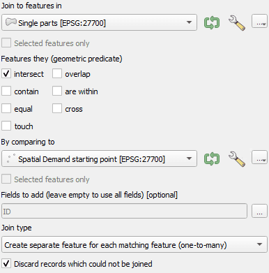
Figure 13: “Join by Location” tool settings used for deleting orphaned polygon fragments

The result of this process is the creation of a new polygon for each interaction between a parent heat demand and a child fragment with which it intersects^[12].

The buffer fragments that pass this check were then dissolved (using the QGIS tool of the same name) to merge overlapping buffer areas into combined proto-opportunity areas.

Joining attributes to polygons and screening by property count

A spatial summary join was performed between the proto-opportunity polygons created in the previous step and the heat demand point data from which they were created. This enabled the polygons to be categorised as ‘opportunities’ or non-opportunities. Summary statistics were calculated to determine the total heat demand for the opportunities, as well as creating a grouping scale indicator similar to that created for Communal Opportunities (the sum of the heat demands’ values if domestic = 1 and non-domestic = 2).

The proto-opportunity polygons were then filtered using a grouping scale indicator threshold of 10. Groupings which did not meet the threshold were deleted.

Trimming of Multi-Building Opportunity and High Property Count Area shapes

The process that creates Multi-Building Opportunity groupings, laid out in previous sections, sometimes results in polygons with highly irregular shapes. A trimming process was applied that cut opportunity areas along the boundaries of Census Output Areas, using the same tools as described in Section 5.5.2^[13]. This action created fragments that belonged to different Output Areas to the rest of the opportunity area but contained no heat demands. These fragments were deleted and the remaining areas (all containing heat demands) were re-joined using the process described in Section 5.5.3. The result was a set of ‘trimmed’ polygons which represented Multi-Building Opportunities. In general, this was a change that impacted the visual representation of the opportunities only (not the groupings of buildings or characterising data, other than the area of the opportunity polygon).

In a small number of cases (138, or 1% of the Multi-Building Opportunities), the trimming process resulted in one or more heat demands being isolated from the grouping that they belonged to. These fragments were deleted from the Multi-Building Opportunity dataset.

Separation of Multi-Building Opportunities and High Property Count Areas

With the final Opportunity areas created and summary statistics joined, a further classification step was completed to differentiate between High Property Count Areas and the Multi-Building Opportunities which form the focus of the national assessment. Using the property count fields added in a previous step, High Property Count Areas were separated from the other polygons whenever the property count was greater than or equal to 1,000.

High Heat Demand Areas were identified within the High Property Count Areas dataset by selecting only those areas with total heat demands above 100,000 MWh per year.

Matching of non-contiguous heat sources to opportunities

Waste heat sources

13 new data centre locations were identified through a web search and added to the waste heat sources dataset from the Scotland Heat Map (without any of the characterising data that is present in the SHM).

Buffer radii were calculated for all waste heat sources using the process described in Section 5.2.2, but this time using a Linear Heat Density proxy of 4,000 kWh/metre/year multiplied by their estimated annual heat supply capacity. Data centres that do not feature in the Scotland Heat Map dataset were assigned a buffer radius of 1 km. Buffers were then drawn in the GIS environment using the process described in Section 5.5.1.

Maximum connection distances were calculated for Communal Opportunities and Multi-Building Opportunities, also using a Linear Heat Density proxy of 4,000 kWh/metre/year multiplied by their total estimated annual heat demand.

A proximity analysis considered the separation between a waste heat source’s point location and either the building footprint of a Communal Opportunity or the geometric centroid of a Multi-Building Opportunity. The centroid was chosen as the evaluation point to avoid instances where ‘limbs’ extending from Multi-Building Opportunity polygons were close to waste heat sources but the majority of the heat demands were not. The choice of the centroid also limited instances where large areas of open green space were within reach of the waste heat source, but heat demands were not.

Using spatial join operations in QGIS, any demand evaluation points (building footprints or opportunity centroids) located within the maximum supply-driven connection distance of each waste heat source were taken forward for further evaluation based on the demand-driven maximum connection distance.

For each waste heat source and opportunity pairing identified through a spatial intersection, lines were drawn between the waste heat locations and the point or polygon representing the opportunity. This was done using the “Shortest Line Between Points” tool in QGIS. Each line represented a potential match between supply and demand, with the line also facilitating the calculation of the distance between the two. These distances were compared against the corresponding demand-driven maximum connection distances previously calculated. Any lines that exceed the maximum distance for their matched demand group were removed from the analysis. Each remaining connection line therefore represented a viable spatial match between a waste heat source and an opportunity.

Waste heat sources that had been matched with low temperature heat network opportunities were processed into a dedicated output dataset which captures their locations and the relevant fields present in the original Scotland Heat Map layer such as the heat source sector and annual supply potential (where available).

Blue and green spaces

The blue space dataset was created by combining Ordnance Survey mapping of static water bodies, waterways and coasts into a single file. This included rivers, canals, lochs and other major surface water features.

The Green Heat in Green Spaces (GHiGs) dataset was produced by Greenspace Scotland specifically to support the identification of opportunities for hosting ground source heat infrastructure in public green spaces, including in connection with heat networks. The country’s mapped green spaces were already subjected to a degree of screening in the preparation of the dataset. An additional screening step removed blue and green space polygons with areas of less than 1,000 m².

Both the blue space and GHiGs datasets were subject to a geoprocessing step that removed narrow parts of the polygons present. This enabled the subsequent process of matching green and blue space with opportunities to avoid creating unrealistic connections (as explained in Section 4.3.2). This was done by applying a negative (inwards) buffer of 5m to the shapefile which will remove any polygon (or part of a polygon) that is narrower than 10 metres. The resultant layer was then buffered again by 105m (positive, outwards) to counteract the initial negative buffer and implement a maximum matching search radius of 100 metres from the boundary of a green or blue space.

A spatial join was then conducted between the blue and green spaces’ buffers and the opportunities (both multi-building and communal) identified in previous steps. Intersections between these features represented matches between heat sources and opportunities.

Identification and characterisation of anchor loads and cooling customers

Public sector anchor loads were identified according to the criteria stated in Section 5.2.2. Non-public sector anchor loads were identified where the field “PUBLIC_BUILDING_FLAG” in the Non-Domestic Analytics dataset had a value of “Not applicable”, and where the “heatdemand” field in the Scotland Heat Map was greater than 200 MWh per year. Both types of anchor load were processed into dedicated output datasets which capture their locations and characteristics that are relevant to the viability of connecting them to a low temperature heat network. (Dataset joins using the anchor loads’ Unique Property Reference Numbers (UPRNs) enabled data from both Scotland Heat Map and Non-Domestic Analytics to be brought together.)

Potential cooling customers existing within Multi-Building Opportunity groupings were identified through application of the criteria set out in Table 21 to the relevant datasets and performing of a spatial join. The type of building, infrastructure or process was included in a dedicated output dataset which also captures the location of each potential cooling customer.

Table 21: Criteria for the identification of potential cooling customers within Multi-Building Opportunities

Characterisation of Communal Opportunities and Multi-Building Opportunities

A range of characterising data fields were joined onto the Communal Opportunities and Multi-Building Opportunities spatial datasets. (Data fields integral to the opportunity identification process – namely, heat demands and domestic and non-domestic property counts – were already present for these layers as well as for High Property Count Areas.)

Characterising data mostly came from the three address-level datasets (Scotland Heat Map, Home Analytics and Non-Domestic Analytics), with some additional spatial data derived from open government sources (Local Authority and Data Zone boundaries, the Scottish Index of Multiple Deprivation and the Scottish Government Urban Rural Classification). The source of each data field in the Communal Opportunities and Multi-Building Opportunities layers is listed in Table 24 and Table 22. Full details of input datasets are given in Section 3.1 of this Appendix.

The Unique Property Reference Number (UPRN) was the data field used to match values from Home Analytics and Non-Domestic Analytics with the heat demand points that derived from the Scotland Heat Map. The vast majority of SHM heat demand points were also present in the relevant other dataset. However, a total of 6,588 (0.4% of 1.5 million) SHM heat demand UPRNs which were part of Multi-Building Opportunities or High Property Count Areas were not present in Home Analytics or Non-Domestic Analytics. This could have been due to incompleteness of datasets, inconsistencies with UPRN assignment, changes of use, or building demolition. A similarly small fraction of heat demands in Communal Opportunities were affected.

Data from the aforementioned sources was summed, counted or formed the input to further calculations (such as percentages of overall totals). For some data fields, a majority (modal) value from the grouped heat demands was calculated. In some instances, the requirement for data to be aggregated to a certain level (to satisfy data protection and licensing requirements) meant that criteria had to be met for a value to be reported. The calculations applied to each field in the Communal Opportunities and Multi-Building Opportunities layers are set out in Table 23 and Table 25.

Where Scotland Heat Map UPRNs were absent from the other datasets, data relating to these heat demands was excluded from the calculations of group characteristics. This explains why occasionally some values do not sum to the totals that would otherwise we expected. Percentage results represent the distribution of characteristics across heat demands that had Home Analytics and/or Non-Domestic Analytics records only.

Some characterising data fields relate to low temperature heat network ‘archetypes’ that may or may not apply to a particular opportunity. These archetypes were defined by the researchers as set out in Table 14, Section 4.2.10. Archetype identification sometimes required spatial joins to be conducted with layers representing heat sources and anchor loads. Other archetypes are defined by opportunity characteristics like area and urban/rural classification.

SHM = Scotland Heat Map, HA = Home Analytics, NDA = Non-Domestic Analytics, GHiGS = Green Heat in Green Spaces. Table continues on subsequent pages.

Table 22: Source of characterising data fields in the Multi-Building Opportunities output layer

SHM = Scotland Heat Map, HA = Home Analytics, NDA = Non-Domestic Analytics, GHiGS = Green Heat in Green Spaces. Table continues on subsequent pages.

Table 23: Calculation of characterising data fields in the Communal Opportunities output layer

Table continues on subsequent pages

Table 24: Sources of characterising data fields in the Communal Opportunities output layer

Table continues on subsequent pages

Table 25: Calculation of characterising data fields in the Multi-Building Opportunities output layer

Quality assurance

Stakeholder engagement provided some high-level quality assurance of elements of the model design, including key assumptions. Data quality risk assessment and responses are discussed in Section 4.5 of this Appendix. This chapter discusses dedicated quality assurance activities carried out in addition to stakeholder engagement and data quality risk assessment.

Researchers’ quality assurance

Quality assurance checks carried out on the model and its outputs included:

• review of model scope, specification and model map;
• review of methodology (this Appendix) for correctness and fitness-for-purpose;
• review of data outputs User Guide for completeness and fitness-for-purpose;
• maintenance of version control;
• review of data outputs:
• units, precision and data type (numbers, text)
• field and layer labelling
• empty data fields, extreme values and distributions within data layers
• checksums
• review of visualisations for readability and accuracy;
• development of Assumptions Log and Quality Assurance Log, including Issues Log and Possible Improvements Log.

Issues noted were either resolved through adjustments to the model or accepted and discussed in the appropriate section of this Appendix.

Scottish Government quality assurance

A meeting was held with Scottish Government representatives during which elements of the model were demonstrated within the QGIS software environment. Questions were posed and answered on diverse aspects of the methodology. Scottish Government representatives also reviewed Sections 2 to 5 of this Appendix and the Assumptions Log.

Potential improvements

The following potential improvements have been identified while developing and implementing the methodology for the national assessment:

• Conducting sensitivity analysis on the Linear Heat Density-proxy assumption to generate an understanding of how the number and scale of Multi-Building Opportunities varies. This could help practitioners decide which opportunities they should focus on, and would help researchers to build the evidence base regarding the contribution that low temperature heat networks could make to decarbonising heat in buildings.
• Investigating the impact of using the same Linear Heat Density-proxy assumption for public sector anchor loads as for all other types of building. If the impact of treating public anchor loads differently is negligible, the methodology could be simplified.
• Incorporating more recently updated heat demand data from Home Analytics, Non-Domestic Analytics or other sources (including the Scotland Heat Map should it be updated). Improving accuracy due to increasing Energy Performance Certificate (EPC) coverage, new data collection and the development of improved modelling methodologies will improve the ability of the national assessment methodology to identify locations likely to be suitable for low temperature heat networks.
• Sub-archetypes (for example, types of Communal Opportunity based on occupancy or building form) could be developed.
• Scottish Water information regarding the location and capacity of wastewater treatment plants would expand the number of potentially viable waste heat sources available to be matched with nearby low temperature heat network opportunities.
• Ordnance Survey building use classes could be used to expand the list of important sources of waste heat beyond those included in the SHM “Potential Energy Supply” layer.
• Research into the waste heat capacity of non-fossil fuelled thermal power stations (e.g. from condensers that form part of the steam cycle) and anaerobic digestion plants could support the expansion of potential sources of waste heat that could supply low temperature heat networks.
• Improvements to the available data concerning green spaces and woodland could improve the accuracy of the matches identified between green spaces and low temperature heat network opportunities.
• Information on the variation of waste heat availability with time (from daily profiles to seasonal fluctuations) would improve confidence in the degree to which demand from heat users on a network can be met from a waste heat source.

How to cite this publication:

Waters, L., Brown, B. and Brown, A. (2026) ‘National assessment of low temperature heat network opportunities’, ClimateXChange. https://doi.org/10.7488/era/7027

© The University of Edinburgh, 2026
Prepared by The Natural Power Consultants Ltd on behalf of ClimateXChange, The University of Edinburgh. All rights reserved.

While every effort is made to ensure the information in this report is accurate as at the date of the report, no legal responsibility is accepted for any errors, omissions or misleading statements. The views expressed represent those of the author(s), and do not necessarily represent those of the host institutions or funders.

This work was supported by the Rural and Environment Science and Analytical Services Division of the Scottish Government (CoE – CXC).

ClimateXChange

Edinburgh Climate Change Institute

High School Yards

Edinburgh EH1 1LZ

+44 (0) 131 651 4783

info@climatexchange.org.uk

www.climatexchange.org.uk

1. 
   

   Grid electricity connections are near-universal in Scotland, with the notable exception of some islands, remote communities and very remote rural properties. The national assessment has not excluded known off-grid locations. We expect that, in the very rare cases that opportunities are identified in such places, most users will be aware of the constraints that apply. More information can be found in Section 4.2.6 of Appendix A. ↑

   
   
2. 
   

   The categories used in this paragraph are those defined by the Scottish Government’s 6- and 8-fold urban-rural classifications. ↑

   
   
3. 
   

   All geospatial data was reprojected to a common Coordinate Reference System (CRS). ↑

   
   
4. 
   

   Where no EPC exists for an address, the developers of the dataset (and those that feed into it) inferred its heat demand by training statistical and geospatial models using the address-level information that is available, combined with local area statistics (such as from neighbours’ EPCs). The production of EPCs itself involves some simple modelling of a property’s heat requirements based on observations made during a physical survey. ↑

   
   
5. 
   

   Shared Ground Loop schemes are a type of low temperature heat network in which the heat source is a ground source heat collector that is shared between multiple distributed heat pumps. ↑

   
   
6. 
   

   The ‘Potential Energy Supply’ layer derives from an assessment of potential sources of waste heat for heat networks in Scotland carried out by Sinclair and Unkaya (BRE) for ClimateXChange (2020). ↑

   
   
7. 
   

   The Green Heat in Green Spaces project was unable to calculate this quantity with sufficient confidence to publish results and was restricted in terms of the contributory data that was possible to share. ↑

   
   
8. 
   

   The concept of what properties ‘require’ in order to enable heat pump installation is not explained. It is unclear whether operating costs, capital costs, space requirements, consumer acceptance or technology availability (among other possible factors) influence judgments of what is ‘required’. ↑

   
   
9. 
   

   Feasibility studies and options appraisals provide evidence that low temperature heat networks can be, but are not always, cost-competitive with existing polluting heating systems. Comparisons of shared ground loop operating costs with individual air source heat pumps (Element Energy, 2023) can also be considered alongside comparisons of air source heat pumps against fossil heating systems such as those provided by Energy Saving Trust. ↑

   
   
10. 
    

    Evidence could not be found in literature to support this quantitative assumption. Johnston et al. (2024) state that in small properties with low heat demands, the capital costs of an air-to-water heat pump may not be economic and alternative technologies should be considered. We infer that heat pumps connected to low temperature heat networks will similarly be uneconomic for properties with low heat demands. The value of 5,000 kWh per year was selected and justified through the development of a simple cost model comparing a Shared Ground Loop scheme connection with electric storage heaters. The model assumed a heat pump capacity of 3 kW (equal to the smallest ground source heat pumps currently on the market), typical per-property installation costs, heat pump grants available in early 2026 (and expected to continue), typical system efficiencies, long-term average electricity prices, maintenance costs and equipment replacement costs. For properties with low heat demands, air-to-air heat pumps can often outcompete electric storage heaters in terms of overall heating costs. ↑

    
    
11. 
    

    Often this issue can be attributed to changes to buildings that took place between the creation of the datasets on which the Scotland Heat Map 2022 was built, and the creation of the versions of Home Analytics and Non-Domestic Analytics used in the National Assessment. Demolitions or changes of use are common changes that would cause this issue. ↑

    
    
12. 
    

    The “Join by Location” tool effectively allows all demands that fall within the spatial boundary of a single parts polygon to share its ID with that polygon, creating a new polygon for each interaction (i.e if a buffer fragment contains 5 demand points within it, 5 polygons with one ID each is added to this new layer). A check is then done which matches the ID which was attached to each heat demand point with the ID attached to each new polygon created by the “Join by Location” process. Any polygon without a matching ID (including if there are no heat demand points within it) was considered an “orphaned” fragment. and deleted from the developing polygons layer. ↑

    
    
13. 
    

    The output area polygons available from National Records of Scotland required to be converted into line data format and buffered by 1 metre to give them physical breadth that could interact with opportunity area polygons. Cut opportunity areas were then buffered by 1.1 metres to allow them to re-connect. ↑

    
    
14. 
    

    ‘Off gas’ refers to a property location being more than 63 metres from the nearest Scotia Gas Network gas distribution pipe. It is not related to the fuel used in that property. Independent gas networks are not included. ↑

    
    
15. 
    

    Long Term Development Statements, Network Development Plans, Heat Maps and Primary Substation Polygons from the two Distribution Network Operators that serve Scotland. ↑

    
    
16. 
    

    ‘MoMu class’ is an archetype group developed by Energy Savings Trust that represents common types of blocks of flats in Scotland. ↑

    
    
17. 
    

    ‘Off gas’ refers to a property location being more than 63 metres from the nearest Scotia Gas Network gas distribution pipe. It is not related to the fuel used in that property. Independent gas networks are not included. ↑

    
    
18. 
    

    Long Term Development Statements, Network Development Plans, Heat Maps and Primary Substation Polygons from the two Distribution Network Operators that serve Scotland. ↑

    
    
19. 
    

    In QGIS, rather than performing a ‘Count’ calculation, it was necessary to sum a field that contained a ‘1’ for heat demands that were to be counted and a ‘0’ for all other heat demands. ↑

    
    
20. 
    

    ‘Off gas’ refers to a property location being more than 63 metres from the nearest Scotia Gas Network gas distribution pipe. It is not related to the fuel used in that property. Independent gas networks are not included. ↑

    
    
21. 
    

    ‘MoMu class’ is an archetype group developed by Energy Savings Trust that represents common types of blocks of flats in Scotland. ↑

    
    
22. 
    

    In QGIS, rather than performing a ‘Count’ calculation, it was necessary to sum a field that contained a ‘1’ for heat demands that were to be counted and a ‘0’ for all other heat demands. ↑

    
    
23. 
    

    ‘Off gas’ refers to a property location being more than 63 metres from the nearest Scotia Gas Network gas distribution pipe. It is not related to the fuel used in that property. Independent gas networks are not included. ↑

    
    

Interactive Energy Performance Certificate (EPC) user interfaces could allow householders to better assess potential retrofit measures, which could in turn prompt households to undertake energy efficiency measures and switch to clean heat systems.

This report aims to inform Scottish Government whether it would be beneficial to incorporate data or functionality into the national EPC register to support potential EPC interactivity.

The research explored a number of existing tools that offer a level of interactivity with EPC-like outputs and also involved a desk-based literature review.

Findings

Three levels of potential interactivity were identified to consider implementing in relation to EPCs:

1. Simple interaction, where no new user data and no integration with a calculation engine are required.
2. Medium interaction, where no new user data is required, but integration with a calculation engine is required.
3. Detailed interaction, where customised user behaviour and occupancy inputs could update outputs via integration with an enhanced calculation engine.

No direct evidence was found to support whether simpler or more detailed interaction is more likely to prompt households to retrofit.

The EPC outputs likely to be most useful to households are costs: household energy running costs, running cost savings, and the capital cost of various retrofit measures. The extent to which these outputs may be customised varies, as does the complexity of implementation.

Customising more variables may not necessarily make the outputs more representative, since the reliability of obtaining some of those inputs may be quite low. At any level of customisation, it will be necessary to inform tool users that outputs are ultimately estimates.

There are a number of existing tools that already deliver energy advice to households, which have varying levels of interactivity and customisation.

Limited evidence was identified of a direct link between the provision of customised information and households being prompted to retrofit. However, various literature sources quoting both professionals and typical consumers call for interactivity and customisation of EPCs. There is also relatable evidence that the provision of tailored information to households can prompt behavioural change. Offering households some level of interactivity alongside a traditional ‘static’ EPC could therefore be beneficial.

For further information please read the report.

If you require the report in an alternative format, such as a Word document, please contact info@climatexchange.org.uk or 0131 651 4783.

Image credit: Photo by Laurentiu Morariu on Unsplash

 Research completed March 2025

DOI: http://dx.doi.org/10.7488/era/6008

Executive summary

This project was commissioned to inform the Scottish Government on the potential for an interactive Energy Performance Certificate (EPC) in Scotland. It is proposed that interactivity could allow householders to better assess potential retrofit measures. This, in turn, may prompt households to undertake energy efficiency measures and switch to clean heat systems. This report will help inform whether it would be beneficial to incorporate data or functionality into the national EPC register to support potential EPC interactivity.

Key findings

Three levels of potential interactivity have been identified for the Scottish Government to consider implementing in relation to EPCs:

1. Simple interaction, where both (i) no new user data and (ii) no integration with a calculation engine are required. Users could choose between customised or simplified views of EPC data. Click-through links signposting to further information could also be included (e.g. about measures, funding, further advice services).
2. Medium interaction, where (i) no new user data is required, but (ii) integration with a calculation engine is required. Users could see updated calculations based on already-completed as well as potential retrofit measures. Fuel costs could be updated in line with recent trends.
3. Detailed interaction, where customised user behaviour and occupancy inputs could update outputs via integration with an enhanced calculation engine (medium interaction functions also included). Users could personalise a range of inputs for which default values are normally applied in an EPC calculation.

The EPC outputs likely to be most useful to households are costs: household energy running costs, running cost savings, and the capital cost of various retrofit measures. The extent to which these outputs may be customised varies, as does the complexity of implementation. For example, household energy running costs could be updated by simply considering the latest fuel prices. Or, it could be tailored by updating one or more of the following variables: fuel prices, occupancy, heating temperature set point, heating patterns, or the number of baths or showers taken per day.

However, customising more variables may not necessarily make the outputs more representative, since the reliability of obtaining some of those inputs may be quite low. At any level of customisation, it will be necessary to inform tool users that outputs are ultimately estimates. Actual energy use and costs will inevitably be influenced by annual climate severity, changing fuel prices, and changes in household circumstances.

There are a number of existing tools that already deliver energy advice to households. These have varying levels of interactivity and customisation. In response to user testing and feedback, many offer relatively limited customisation. Circumstantially, this supports the reasoning that a modest spectrum of customisation may be the limit to which users are prepared to use such tools.

Limited evidence was identified of a direct link between the provision of customised information and households being prompted to retrofit. However, various literature sources quoting both professionals and typical consumers call for interactivity and customisation of EPCs. There is also relatable evidence that the provision of tailored information to households can prompt behavioural change. Offering households some level of interactivity alongside a traditional ‘static’ EPC could therefore be beneficial. Unfortunately, no direct evidence was found to support whether simpler or more detailed interaction is more likely to prompt households to retrofit.

Considerations for implementation

If the Scottish Government is minded to pursue an interactive tool, there are various options. It may commission its own interactive tool, or alternatively, it may look to use or adapt an existing tool to deliver a similar service.

The Scottish Government will also need to consider how best to integrate net zero policy ambitions in the implementation of any tool outputs or recommendations.

Providing sufficient interaction/ customisation for end users to feel that outputs are relevant to them is likely to be most important. The ability to update information from a ‘static’ EPC to reflect changes that have already taken place will likely be key. Furthermore, the ability to toggle retrofit measures will give users a sense of choice and control.

While a relatively simple implementation may suit the majority of potential users, a minority of users may see particular benefit in tailoring a wider range of input variables. If ‘detailed interactivity’ were implemented (as defined above), then customised views/ functions for different user groups may help simplify the user experience.

Glossary / Abbreviations table

Introduction

This project considers how an interactive Energy Performance Certificate (EPC) user interface may help to increase public uptake of energy efficiency and clean heating options in homes.

There could be an opportunity to integrate data that would support the development of an interactive EPC user interface when assessing the future needs of the national EPC register in Scotland. A system that enables the public to better assess energy efficiency and clean heat options may be expected to increase uptake of these measures. However, the Scottish Government needs to understand the likely benefits and limitations of such an interactive user interface before it makes decisions on changes to the EPC register.

Background and research scope

The focus of this report is on domestic EPCs. An EPC assessment combines findings from a physical survey of a building with standardised assumptions on how it is used. EPCs therefore provide an ‘asset performance assessment’ that allows homes to be compared to others elsewhere in the country. This is regardless of whether they are different sizes, specifications, or have different systems and/or use patterns. They are accompanied by a Recommendations Report. This provides examples of measures that may improve the efficiency of the home and make savings, intended to encourage homeowners to take action. Recommendations are presented in a set sequence that follows a fabric-first approach, with renewable energy sources considered last. EPCs are therefore an important source of information for homeowners and buyers to inform decision making.

However, the presentation of recommendations and savings means users are not aware of the impacts of implementing measures out of sequence. Also, EPCs do not provide information regarding potential options for switching to cleaner heat systems where properties are currently served by another fuel type. EPCs as therefore not necessarily aligned with the aims of the Scottish Government Heat in Buildings Strategy with regard to clean heat systems. Savings predictions reflect the standardised assumptions made in the EPC calculation in relation to occupancy and heating patterns. This makes the EPC less helpful when a homeowner wants to understand the benefits and savings they may experience according to their own circumstances. Offering users a level of interactivity may allow benefits of different potential improvement measures to be expressed. This can lead to more tailored recommendations and thus may better support users to act on them. There could therefore be value in a traditional ‘static’ public EPC for regulatory compliance, and an interactive interface to provide customisation for homeowners.

The scope of the research was therefore to identify the data inputs and outputs that may be relevant to an interactive EPC and consider how data inputs may be sourced.

The focus was on interactivity that would allow homeowners to input contextual information about how they use their home; essentially customising aspects of the EPC calculation that would otherwise use standardised assumptions, e.g. occupancy, heating patterns and temperatures. It was assumed that data obtained from an original EPC building survey would not fundamentally be challenged, e.g. floor areas, construction types. However, it is acknowledged that homeowners may wish to update information where retrofit works had already taken place since the EPC was carried out. For example, when new insulation has been installed or when energy systems have been upgraded or changed. Note that implications of the General Data Protection Regulation (GDPR) on interactive EPCs were deemed beyond the scope of this study.

Further, we sought evidence to understand the benefits and limitations that an interactive EPC interface may provide, to demonstrate whether user interactivity has led to increased uptake of retrofit measures. Our research explored a number of existing tools that offer a level of interactivity with EPC-like outputs. These were primarily targeted at homeowners (i.e. covering domestic/ residential properties), although portfolio-level tools were also briefly considered. The research also involved a desk-based literature review.

Data inputs and outputs for potential EPC interactivity

EPC review

Domestic EPCs for Scotland are produced using the UK Government’s Standard Assessment Procedure (SAP) implemented in approved software tools. For existing dwellings, it is recognised that detailed construction information is unlikely to be available. A ‘reduced data’ version of SAP (RdSAP) is therefore used, which makes assumptions about the construction based on age, etc. A selection of the inputs and outputs of the resulting calculation are held centrally in the Scottish Government’s EPC Register. Note, however, that not all intermediary outputs from the RdSAP calculation steps are held on the Register.

EPC outputs

We reviewed the outputs reported on a current Scottish domestic EPC (as at 2024). Those that may be relevant to end users making decisions on energy efficiency and clean heat measures were identified, as noted below. Further metrics proposed in the Scottish Government consultation on EPC reform were also considered for insight into potential future changes.

• Energy Efficiency Rating (EER) (also known as the ‘SAP score’; Proposed to be called ‘Energy Cost Rating’ following EPC reform)
• Environmental Impact Rating (EIR)
• Primary energy indicator (kWh/m²year)
• Running costs (£ for 3 years)
• Savings (from potential recommended measures) (£ for 3 years)
• Savings per recommended measure (£ for 3 years)
• Recommended measures capital cost (£)
• Emissions from the home (kgCO₂/m²/year)
• Space heating demand (kWh/year)
• Water heating demand (kWh/year)
• Heat Retention Rating (proposed for EPC reform; expected to be similar to Space heating demand metric)
• Total energy use (proposed for EPC reform; expected to be similar to the calculation for primary energy indicator, but for delivered energy, i.e. without primary energy multiplier)

Dependent inputs

We then interrogated the underlying RdSAP calculation methodology^[1] to identify the key inputs used to calculate the identified outputs. All outputs are derived from numerous inputs and calculation steps, with the exception of ‘Recommended measures capital costs’, which are simply quoted reference values. Inputs that offer the potential for contextual customisation relevant to particular occupant behaviour/use are noted below.

• Fuel prices and standing charges
• Capital costs for retrofit measures
• Number of occupants
• Number of baths or showers taken per day
• Living room comfort temperature set point
• Heating pattern on/off times (for a normal day and an alternative day, e.g. weekend)
• External temperature (from regional climate information)

Ease of implementation

We made a qualitative assessment of the ease with which the above EPC outputs may be customised via calculation. Extensive customisation of an RdSAP calculation using occupancy parameters was implemented in the Green Deal Occupancy Assessment (GDOA) tool^[2]. Since the GDOA tool functionality already exists^[3], customisation of a number of contextual/ user inputs could be relatively easily facilitated in an RdSAP 2012 calculation. The following ‘ease of implementation’ ranking was therefore applied to the EPC outputs identified above:

• High ease: Where an output already held on the Scottish EPC register could be adapted via a straightforward side calculation (i.e. where no RdSAP calculation engine would be required to re-model the impact).
• Medium ease: Where the output could be updated by implementing aspects of the GDOA as part of a new RdSAP calculation, using data held on the EPC register.
• Low ease: Where customisation of metrics has not previously been implemented in an RdSAP calculation, and therefore more work would be required to implement.

Note: In assigning this ‘ease’ hierarchy, it is assumed that the data held in the non-public version of the Scottish EPC register aligns with the import requirements of an RdSAP 2012 calculation. This appears likely to be the case based on summary information provided by the Scottish Government for this study. However, this would need to be verified in order to validate the recommendations of this study.

Table 1 shows the qualitative ‘ease of implementation’ ranking for customised EPC outputs.

The table refers to the SAP Product Characteristics Database (PCDB). The PCDB holds reference data for mechanical systems, which is used in SAP and RdSAP calculations. It also holds fuel prices and estimates for the capital costs of measures that are used in RdSAP calculations. Fuel prices are updated in the PCDB every 6 months but they are fixed in an EPC at the time of its issue. Capital cost of measures are only updated when a new version of the RdSAP methodology is released.

Currently, the EPC register does not store fuel use totals from the RdSAP calculation, although it is an intermediary calculated value that underpins many subsequent metrics. It is understood that this data is absent from both the public and non-public versions of the register held by the Scottish Government. It follows that even relatively simple-seeming amendments to EPC outputs, e.g. updating fuel prices, would require an RdSAP calculation to be re-run. Two scenarios have been presented in Table 1 for ‘Recommended measures capital cost’. Scenario A is assigned a ‘high’ ease of implementation, while Scenario B is assigned a ‘low’ ease of implementation. The measures costs applied to an EPC are generic and not tailored to the property (e.g. according to property dimensions, or similar). Scenario A assumes this is still the case but an alternative, updated source for measures costs could be referenced by an interactive tool. Customised retrofit measures costs were not a function that was implemented in the GDOA. Therefore, if such a customisation function were desired, this scenario would have a low ease of implementation.

Table 1: Ranking of current and proposed EPC outputs according to their anticipated
ease of customisation

End user value of existing EPC outputs

The EPC outputs identified in 5.1.1 were qualitatively assessed for their likely importance to end users in retrofit decision making. Discussions were held with Retrofit Coordinators at the National Energy Foundation, who directly engage with households on energy retrofit. Their feedback is supported in various studies (including National Retrofit Hub (NRH), (2024), Which? (2024), Jones (2022), and Bančič, Vetršek and Podjed (2021)) that have examined which metrics different end users find or would find valuable when considering home upgrades. In Table 2, the EPC outputs have again been assigned a ranking, this time indicating their expected usefulness to end users. Notes provide supporting rationale for each ranking.

Table 2: Ranking of EPC outputs according to their likely importance to end users
in retrofit decision making

Simple cost-based metrics are more likely to be easily understood by consumers and are therefore more likely to contribute to retrofit decision making. This includes running costs and cost savings from potential retrofit measures. Energy assessors, consultants or other professionals in the sector may see value in the other metrics, but feedback suggests these are of less use to households. Furthermore, the concept of carbon emissions is identified in the above reference sources as not being tangible for most consumers, despite national policy striving for ‘net zero’.

Review of existing interactive home energy advice tools

Numerous tools are available, beyond a traditional RdSAP calculation, that offer EPC-type outputs to users with a level of interactivity/customisation. A selection of these tools were reviewed for this study to consider the possible forms a Scottish EPC user interface could take. Tools were identified using web searches and the knowledge of the research team. Criteria for inclusion included:

• A domestic/ housing focus
• An aspect of interactivity/customisation
• Outputs similar in nature to those on an EPC (e.g. energy use, cost, retrofit recommendations)

Six tools were then selected for more detailed investigation. Selection criteria included:

• Sufficient information available so they could be assessed for this research
• Tools offering differing levels of interactivity/customisation
• Limiting duplication of tools created by a single organisation, unless they offered something distinctly different from one another
• Inclusion of a commercial/ portfolio assessment tool

We assessed outputs provided by each tool and the customisable inputs they request from users. These are summarised in Table 5 and Table 6 respectively, in Appendix A, alongside the outputs and inputs discussed earlier for EPCs. For the latter, the potential inputs are those of the RdSAP Green Deal Occupancy Assessment, which is taken as a baseline for calculation customisation potential.

It is apparent that many consumer-facing tools are based on a limited number of calculation engines. The Energy Saving Trust (EST) engine and the Parity Projects/ Core Logic engine appear to be popular options underpinning branded tools. These front-end tools may offer slight variations in presentation or user functionality, but they draw on the same foundational data and calculation approach. All tools rely on an underlying RdSAP calculation engine to generate outputs. However, they do not offer the full functionality of RdSAP to be customised, instead utilising many assumptions and generalisations. Most tools use at least some EPC data (from the EPC register) to pre-populate information for calculations.

Tools typically offer one or more of the following levels of interactivity/customisation:

• Ability to toggle potential retrofit measures on or off and assess impacts/ benefits
• Ability to make simple updates to property data (compared to that held on EPC), e.g. if insulation or new windows have been installed. Some also ask if there is space to facilitate renewable energy systems
• Ability to provide basic contextual or occupancy information (some tools will typically progress with assumptions if users do not wish to provide customised information e.g., number of occupants, typical living room set point temperature, when people are typically at home)
• Ability to provide more detailed contextual or occupancy information (again, some tools will typically progress with assumptions if users do not wish to provide customise information e.g., number of baths and showers taken per week, actual energy use totals from bills)

Many tools also offer further interactivity that does not relate to the calculations process but provides users with additional information. Examples include click-through links providing:

• Specific information about retrofit measures
• Information about potential funding or finance options
• Links to trusted trades or advisory services (e.g., TrustMark, one-stop-shops)
• Links to professional whole house retrofit plan or Retrofit Coordination services

It was noted in discussions with NEF that consumers often feedback that they are not confident translating a retrofit plan into action. There is apparently often distrust of trades/ contractors. Qualitative information such as that above may help households build confidence to take plans forward.

None of the consumer-facing tools reviewed allows for customisation to the same extent as the GDOA tool. The EST/ Home Energy Scotland tool provided the widest range of user customisation options. From discussions with a selection of tool owners, their user testing and feedback has identified a need for relative simplicity. It is assumed that this reasoning has also been applied to other tools, as they often offer similar functionality.

All the reviewed tools focus on the outputs expected to be of most value to consumers, as noted in section 5.1.4. These include running costs, cost savings from measures and the expected capital cost of retrofit measures. Most tools also report associated carbon emissions. However, despite this alignment in key outputs, the extent to which inputs can be customised varies across tools. It may be expected that outputs based on more extensive customisation will be more representative of a user’s actual circumstances. It is relatively unlikely that users will have an appreciation of this though, since they may only ever interact with one tool. All tools evidently have their place in the market, though it is very difficult to accurately assess their respective ‘success’ (i.e. the extent to which they encourage homeowners to undertake retrofit). Some commentary is offered in relation to specific tools below.

A consistent aspect of functionality offered across all tools is the ability to update whether some building elements have already been enhanced. They all also offer the option to select different potential retrofit measures to form a tailored retrofit plan. It should be noted however, that these outputs are not equivalent to a ‘whole house retrofit plan’ as defined by the PAS 2035 framework (BSI, 2023). These aspects of interactivity can help consumers consider the impacts of certain retrofit options and thus they can provide a useful step beyond a traditional ‘static’ EPC. It may be inferred that these are the aspects of most value to consumers, and there is perhaps less focus on perceived ‘accuracy’ of further customisation. Some aspects of the reviewed tools are discussed in more detail below.

UK Government ‘Find ways to save energy’ tool

This tool is owned by the Department for Energy Security and Net Zero (DESNZ). It uses an RdSAP engine hosted by BRE that implements selected parts of the GDOA. It includes default assumptions being made for parts of the GDOA that users are not asked to customise. DESNZ have indicated in discussions that user testing and consumer feedback has shaped the current functionality of the tool. For example, an earlier release of the tool included more customisation questions. However, these were removed as they led to high levels of user ‘drop out’ associated with those questions (i.e. users exited the online tool without completing beyond certain questions). Additional feedback suggests that a minority of users (estimated ~10%) would like more detail than the tool currently offers. DESNZ are exploring options for potential future updates.

EST engine backed tools

Three different tools were reviewed that utilise EST’s calculation engine:

• Home energy check (branded as Home Energy Scotland)
• Go renewable tool, developed with the Microgeneration Certification Scheme (MCS)
• The Snugg Plan Builder (an example with a custom branded front end)

Each offers slightly different functionality and very different user interfaces. For example, the Home Energy Scotland tool does not directly link with the EPC register. However, users are encouraged to obtain their EPC information (from the register if not readily available) to aid answering questions. The Go renewable tool, as the name suggests, focusses on advising on renewable energy systems. It also gives recommendations on basic fabric efficiency measures that should ideally be carried out in conjunction with certain renewables.

Go Renewable and the Snugg Plan Builder each introduce some novel output metrics. Go Renewable offers a ‘heating system running cost metric’, which allows different heating system options to be directly compared. The Snugg tool features a metric on the potential income from a PV system (based on the Smart Export Guarantee). It also estimates a potential increase in property value increase resulting from installing retrofit measures. ‘Savings’ metrics may not motivate landlords or people that do not expect to stay in a home that long. However, metrics linked to property value may be an alternative motivator for such users.

Parity Project/ Core Logic ‘EcoRefurb’ tool

EcoRefurb is part of the Core Logic ‘Plan Builder’ suite of tools. It is an example of a branded front-end tool that uses the underlying Core Logic engine. According to the developers, user testing shaped the development of both inputs and outputs within the tool. One key aspect they identified as important was the provision more customised measure recommendation costs for users. Very few users apparently fed back that they would like to get into more detail in the initial assessment. More detail may be customised in the Plan Builder tool Core Logic provide to Retrofit Coordinators (similar to that in the GDOA) however, this was not reviewed during this study.

IRT ‘DREam’ stock assessment tool

Stock-level assessment tools were also considered during this study, although it is acknowledged that householders are not their target end users. The IRT tool is one such example intended for housing providers^[4] (e.g. social landlords) to assess potential retrofit options at a stock level. Customisation typically focuses on filling data gaps where individual property surveys or EPCs have not been conducted. They also allow updated information to be input, based on maintenance records for example, to provide updated energy data for properties. A key feature of the DREam tool is that it integrates a map function and can overlay areas by index of multiple deprivation for example. It also provides comparisons of funding options that may support housing providers to deliver area based retrofit schemes. Understandably, occupancy-based customisation is not a focus of tools such as this. However, the property information updating and measures toggling functions are evidently important interactive outputs for the tool’s target audience.

Discussion: Levels of interactivity

Three broad levels of interactivity (simple, medium and detailed) are identified here for potential application to the existing EPC, for consideration by the Scottish Government. These levels reflect the functionality of the calculation tools that underpin an EPC and the capabilities of other existing interactive ‘energy advice’ tools that have been reviewed. This also assumes that data from the non-public version of the Scottish EPC register is sufficient to recreate a new RdSAP 2012 calculation for a dwelling.

Simple interaction

This is characterised as interaction that requires no new user data to be input and no calculation engine. Examples of potential functionality could include:

• The ability to provide switchable, customised or simplified views for data for different types of user via an online interface. For example, more detailed EPC information could be accessible by professionals, while only key outputs may be required by households, with options to switch between views.
• Click-through links signposting users to further information – such as details about measures or funding, links to trusted tradespeople or advisory services, etc.

Medium interaction

At this level, no new data inputs are required from users, but an RdSAP calculation engine would be needed to support provision of increased interactivity. Examples of potential functionality could include:

• Allowing users to select their own potential retrofit measures, providing tailored cost savings for different retrofit approaches or combinations of measures (rather than a fixed sequence as per the current EPC methodology).
• Enabling potential updates to property information where retrofit measures have already been installed.
• Incorporating updated fuel costs sourced from the latest version of the PCDB.

Detailed interaction

Here it is assumed that a calculation engine is capable of incorporating customised user inputs to inform updated outputs. (All of the medium interaction functions above should also be possible at this level.) Examples of potential customisation could include updating with:

• Actual household fuel costs and standing charges.
• Actual number of occupants.
• Actual living room temperature set points, heating schedules.
• Actual number of baths or showers taken per day by household.

Section 6 discusses the ease with which data inputs may be sourced. It highlights that there may be a sliding scale of complexity of customisation at the ‘detailed’ level.

Implications related to RdSAP 10 and the Home Energy Model (HEM)

Data currently held on the Scottish EPC Register will have been created using the RdSAP 2012 software version. Reusing this data to re-run a new RdSAP calculation will therefore be more straightforward with an RdSAP 2012 engine. This is subject to confirmation that data held in the non-public version of the register is an appropriate format.

An updated version of the software, RdSAP 10, is currently in development. The ‘full’ version of SAP 10 has been in use since 2022 for newly built homes. It introduces several updates, related to heat pumps and introduces battery storage into calculations.

Translation of existing EPC Register data (created under RdSAP 2012) for use with a newer SAP engine such as the proposed RdSAP 10 would be more complex. Additional assumptions would need to be added alongside the original data from the EPC register. Furthermore, there is also no GDOA implementation in RdSAP 10 (i.e. customisation of occupancy parameters), so a further exercise would be required to replicate this functionality. However, moving to an RdSAP 10 engine would bring any new tool in line with the most current calculations, based on updated research.

The Home Energy Model (HEM) is a new calculation methodology that will eventually replace SAP and RdSAP. A key change in this approach is that calculations will be performed with much finer time resolution. While existing SAP and RdSAP calculations consider a monthly timestep, HEM utilises a 30-minute resolution. This is expected to better-represent heating demands, energy storage and demand flexibility potential for example.

HEM is based on a fundamentally different underpinning architecture compared to SAP. It will use ‘wrappers’ to assess different use cases, with each wrapper defining inputs and outputs that are processed by the core HEM model. One such wrapper will support the Future Homes Standard (FHS). In this context, key changes to modelling assumptions are expected compared to SAP. For example, assumptions about occupancy being linked to floor area (as in SAP) to being based on the number of bedrooms in a property. These changes reflect evolving consumer behaviours and systems operation patterns, highlighting further divergence from the assumptions used in SAP 10.

HEM will undoubtedly offer additional functionality compared to SAP, along with the ability to assess certain technologies more effectively due to its increased granularity. Some innovators, such as City Science and Furbnow, are already attempting to link existing home energy assessments to HEM. Both have undertaken projects in this space with the support of Innovate UK. However, during presentations at the Innovate UK ‘Net Zero Heat Open Day’ both organisations reported that additional input data, gathered from surveys and/or monitoring, is needed to achieve this (UKRI, 2024). That being the case, it seems unlikely that data from the existing EPC register could readily be aligned with HEM. Exploring the effort likely required in achieving this was beyond the scope of this study.

Data collection/ input methods and limitations

Review of potential data sources

A number of potentially customisable data inputs were identified in section 5.1.2.^[5] This section explores ways such data may be sourced and/ or physically input into a tool (e.g., automated versus manual methods). While several theoretical options have been explored, the likelihood of some such information being available/ usable short term is low.

Table 7 in Appendix A gives an overview of relevant data input options that were identified during this study. Each input method was qualitatively assessed, based on the research team’s judgement, on a ‘high, medium, or low’ scale against the following parameters:

• The ease of data input for the user
• Likely reliability of the information
• Likelihood of an information source to be available in the short-to-medium term

The rankings were assigned a score (High = 3, Medium = 2, Low = 1). These were summed to provide an overall current ‘readiness’ metric (scored out of 9).

Manual data entry approaches

Manual approaches rely on households obtaining data from existing sources (such as energy bills) or simply recalling their comfort/ heating preferences (e.g. temperature set points and heating patterns). Users will also readily know how many occupants are typically in the house.

The current readiness score of some manual inputs reflects the potential risk of reduced reliability when households need to consider typical conditions over a whole year. For example, if users never adjust temperature set points on their thermostats, reliability of temperature inputs may be high. This may also be the case if they never adjust programmed heating patterns. However, users are unlikely to take account of incidental day-to-day or seasonal adjustments made outside the normal programming. It is also unlikely that households would consistently track their average number of baths and showers per day for a whole year. A best estimate based on typical patterns seems far more likely. Reliability of some inputs may therefore be low when it depends on household recollection rather than on actual recorded data.

Automated data entry approaches

Automated methods range from updating information from the PCDB through to potentially obtaining data from internet of things smart devices. Fuel prices and standing charges could be taken from the most recent version of the PCDB. There are artificial intelligence (AI) tools that exist (generally intended for businesses) that can extract information from digital energy bills. However, for individual households, such tools are unlikely to be warranted since the information could manually be obtained relatively easily. Smart sensors include motion detectors (inferring occupancy), shower sensors, thermostats and programmers. All of these devices may theoretically be able to track and log conditions and output household data.

Note that there is currently no function or API (Application Programming Interface) to import external data sources into an RdSAP calculation. SAP calculations call on data held in the PCDB, but this database is updated periodically and not accessed ‘live’. The automated transfer of data is therefore an aspect that would need to be developed, if such functionality were desired. Subsequently, any proprietary sources of data (e.g. from consumer apps) would need to be collated and formatted accordingly to feed into SAP. It is assumed that users would be unlikely to manually process such data themselves if it were not automatically formatted and exported.

Automated methods therefore tend to score less highly than equivalent manual methods in the combined readiness metric. They score highly with respect to the ease of data input for the user and many provide inherently reliable data. However, they score low on the short-term likelihood for such automated functionality to be available. Fuel prices updated automatically from the PCDB are assumed to be less reliable than actual data from household bills due to averaging. However, the relative ease of implementing such an update still gives a high overall readiness score (8 out of 9).

Discussion of external temperature data

The RdSAP calculation utilises climate data broken down into 21 UK regions. These include assumptions for monthly average external temperatures. It is possible that some users may question whether the granularity of these climate zones is representative of their local conditions. However, it is quite likely that most users would not have the necessary awareness to challenge the relative accuracy of the climate data used.

Monthly temperature data is available from the MET office (the source of the current RdSAP climate data) at a resolution of 2km. This is a far higher resolution than the 21 UK regions. The format is essentially the same as is used in an RdSAP calculation. However, it would require reasonable effort (and signposting) for users to obtain this data manually and enter it into a user interface. As discussed above for automated methods, there is currently no function for new data to be imported into RdSAP. This would need to be specifically developed to automate the input of new, more granular external temperature data.

Something of potential interest to users and the Scottish Government is that the MET Office also provide ‘future climate scenario’ data sets. If incorporated into an RdSAP calculation, it would be possible to see the impact of changing climate conditions on key outputs and recommendations. Granularity varies depending on the type of climate predictions offered. For example, monthly average temperature predictions against the highest emission scenario (RCP8.5) are projected at a 12km scale. Import of such data to RdSAP would face the same challenges as other updated MET Office data noted above.

Varying interactivity options for outputs

Table 3 shows the outputs assessed as being of highest importance to consumers^[6] alongside the relevant potentially customisable inputs. ‘Emissions from the home’ is also included, since the policy focus of retrofit is ultimately on achieving net zero emissions. Both a ‘medium interaction’ and ‘detailed interaction’ version (as per section 5.3) is included where such options exist. Note the medium interaction would require a SAP calculation engine but no new user input, instead using updated information from the PCDB or elsewhere. The highest ‘readiness’ levels determined for each of the data inputs is presented in the table.

Table 3: Highest ‘readiness level’ of data inputs that may be customised for
EPC outputs (at varying levels of interaction)

While some outputs in Table 3 have several potentially customisable inputs, not all may necessarily be customised. The example tools reviewed in section 5.2 implement different customisable inputs yet deliver essentially equivalent outputs. The inputs therefore represent a sliding scale of potential customisation.

Users may find it quite easy to customise one or two inputs with a high-scoring readiness indicator. Meanwhile, a more bespoke version of the same outputs may be possible, but the ease with which the data may be reliably obtained may be lower. This creates a potential risk of dubious accuracy; an output may seem to be accurate since it is based on multiple user customised variables. However, those variable values themselves may be inaccurate or unreliable, thus reducing the overall representativeness of the output. A sensitivity analysis on this phenomenon is unfortunately beyond the scope of this present study.

Absolute accuracy may not in fact be so relevant for an interactive tool intended to aid retrofit decision making. Pre- and post- retrofit energy performance of homes is relative; after all, many variables out of a user’s control influence energy consumption and cost over a given year. (e.g. external climate, energy price changes, varying household needs.) Providing sufficient interaction/ customisation for end users to feel that outputs are relevant to them is likely to be most important. The ability to update information from a ‘static’ EPC to reflect changes that have already taken place will likely be key. The ability to toggle retrofit measures selection will give users a sense of choice and control. Other input variables may be of more or less interest to users depending on how far they feel their behaviours are from ‘typical’. Households that align with these national trends may see little variation in customised calculations compared to default calculations. It is only when household characteristics are quite different from national trends that it may make notable differences to retrofit recommendations.

Evidence of intended outcomes

We looked for evidence that directly linked the use of interactive tools to the initiation of retrofit measures. Information was also sought on whether different types of interaction or customisation were more likely to prompt household decision making. A desk-based evidence review sought information from academic articles and grey literature. A selection of search terms were initially used, as detailed in Appendix B. These were expanded upon as other terms and concepts were identified in the reviewed sources.

In addition, advisors from NEF provided general feedback based on their experiences of directly supporting consumers with retrofit projects and administering grants.

Feedback related to the use of existing interactive energy advice tools, such as those discussed earlier, was also explored. This was primarily via online sources, though interviews were conducted with tool developers where possible. DESNZ (as owners of the UK Government ‘Find ways to save energy’ tool) and Core Logic (EcoRefurb tool) provided direct feedback on their respective tools.

The evidence review was widened to ‘relatable activities’ when it became clear that limited information was available on interactive tools and retrofit. Relatable activities were defined as those in which the provision of some form of customised information prompted behavioural change. The scope was limited to households and housing, and to at least energy-related behaviours, if not retrofit specifically. This broader search was not exhaustive but was intended to provide indicative context relevant to the primary concept.

Review of literature

Many sources suggest there is a need for interactivity and customisation of EPCs, with inference that this could promote the uptake of retrofit measures. However, no evidence was identified in the literature review to confirm that interactive tools would, or have directly, prompted retrofit actions. Nor did the literature review indicate what level of interaction or customisation might be more likely to prompt households to undertake retrofit.

Several EU research projects have explored ways that EPCs could be improved to better-serve various end uses (e.g. U-CERT, D2EPC, X-Tendo, CHRONICLE, EDYCE, Smart living EPC). U-CERT produced an extensive series of recommendations for EPCs (Bančič, Vetršek, and Podjed, 2021). This followed interviews and focus groups with different types of potential EPC users across 11 participating EU countries. Some recommendations related to improved granularity of calculations and reducing the ‘performance gap’ by using dynamic simulation and the use of measured data. However, many specifically focus on helping users better understanding energy use and prompting retrofit action. Several of these are also recognised in other sources (discussed below).

Example recommendations include:

• Focus on cost-based metrics, as these are most tangible for users
• Offer interactivity to make the information relevant to a user’s own circumstances and context
• Provide different views tailored to the needs and knowledge levels of various users:
• (a) non-professional users, for buying and selling properties, for energy management, and for retrofit recommendations.
• (b) Professionals and more advanced users with more detail and technically specific data.
• Digitalisation offers the potential for a ‘modular’ approach from basic to expert with options according to user interests
• Explain the context of assumptions, so users understand if their patterns are likely to be different to what is assumed

Various studies have investigated the extent to which current static EPCs motivate users to retrofit. A recent study by Which? (2024) indicated that EPCs are rarely used to inform renovation decisions. Users instead rely on advice from builders or their intuition. The study suggests that the current format of EPCs does not effectively encourage homeowners carry out energy efficient home improvements, nor does it meaningfully guide their choice of measures.

The D2EPC research study found that less than 5% of end users were motivated to retrofit because of their EPC (Panteli and Duri, 2021). At least half of those surveyed were also not convinced that their EPC accurately represented their building’s energy efficiency. A Barclays/ Ipsos survey (Barclays, 2023) suggests that over half of homeowners do not feel confident making homes more energy efficient. A further study (Hiscox, 2018) indicates that a third of those surveyed renovated to keep up with current trends rather than for functional reasons.

The U-CERT and Which? studies indicate there is a need to update an EPC so they can still be relevant if some changes/ improvements are made. Otherwise they are readily obsolete (Bančič, Vetršek, and Podjed, 2021; Which?, 2024). The Which? study also states that EPC recommendations are too rigid, presented in a specific order rather than tailored to household priorities and budgets. This need for greater flexibility was echoed in discussions with Retrofit Coordinators at NEF who work directly with consumers. They observe that many households are favouring less disruptive, less risky technologies, rather than deep energy efficiency retrofit measures. App-linked technologies also gaining popularity, raising people’s interest in things like heat pumps, PV and battery storage.

This supports a case for savings forecasting across a flexible sequence of measures, rather than the pre-defined order used in EPCs. However, NEF note the importance of linked guidance (i.e. simple interactivity) on risks and implications of implementing measures outside a validated sequence. They advocate the role of Retrofit Coordinators in developing whole house retrofit plans to help households avoid unintended consequences. The U-CERT recommendations similarly stress the value of contextual information and guidance alongside an EPC (Bančič, Vetršek, and Podjed, 2021).

The majority of reviewed literature generally supported the concept of interactivity for EPCs. However, in the experience of innovators ‘Furbnow’ (UKRI, 2024), some users were not confident in entering property data in EPC tools. For this study, we recognise that there is a risk that too much complexity could deter users. Simpler interactivity may therefore be preferable.

Review of relatable activities

The literature review was widened to ‘relatable activities’ based on the research team’s experiences in the energy and retrofit sector. This included exploring links between interactive outputs and intended behavioural change on retrofit plans, smart meters and green finance (for retrofit). Reviewing these relatable activities provided some evidence that customised and/ or interactive information can prompt intended behavioural change among households.

Retrofit plans

Retrofit plans are bespoke reports intended to guide owners on how to retrofit their homes. These follow the principle of considering the individual context of a retrofit, (e.g. user influence), i.e. they include customised recommendations. Building Passport trials (including renovation plans) have been in place for a number of years in several countries and have also been the subject of previous ClimateXChange research (Small-Warner & Sinclair, 2022). Despite this, no quantitative evidence was found that their implementation increases retrofit uptake. Only circumstantial evidence of ‘intent’ from end users was given, suggesting likely future uptake of measures. In other words, it is not currently possible to directly link the implementation of renovation plans in Building Passports to a measurable increase in retrofit.

In the iBroad project trial, the majority of respondents agreed that a renovation roadmap enables and motivates them to undertake retrofit measures (Irish Green Building Council (IGBC), 2020). Similarly, 63% of experts surveyed for the follow-up iBroad2EPC project believed that tool would motivate homeowners to renovate (Mellwig, Maiwald, and Pehnt, 2024).

It was observed that renovation plans implemented in EU countries generally follow national policy by prioritising energy efficiency recommendations before renewable energy measures (Enefirst, no date). This is similar to the current approach taken in UK EPCs. As implemented, these plans do not necessarily provide the flexibility called for in many discussions of EPC reform. They are however, tailored to personal circumstances based on assessor expertise.

Smart meters

Smart meters serve multiple purposes. These include accurate billing, supporting the use of flexible tariffs, and improving visibility of the granularity of energy use at a local and national level. Alongside in-home displays, smart meters provide information that can help households to understand and potentially reduce their energy use.

A study for Smart Energy GB (Populus, 2019) found that consumers with smart meters report a higher number of energy saving activities than non-users. These activities increased over time with continued active smart meter use. There were also increased levels of behavioural change, such as buying more efficient appliances and implementing energy saving habits. Smart meters also enabled people to take part in flexibility and Time of Use activities to save money. These benefits are attributed to the in-home display showing energy use in near real time. This tailored, real-time information was reported to aid users in identifying energy usage and making more informed decisions to reduce usage.

These findings are supported by several other studies, some of which highlight the importance of displaying data in terms of cost to make it more relatable to users. (Darby et al, 2015, National Centre for Social Research (NatCen), 2022, Marshall Cross et al, 2019).

Detailed data (i.e., at appliance level information) was found to be most useful and persuasive for end users. For example, Scottish Power data analysis of interactive app users suggests a 5% energy saving compared to non-users. This is attributed to the more detailed breakdown of energy use, which raises awareness among householders and prompts action (Scottish Power, no date).

These findings support the concept that the provision of bespoke, time-relevant and cost-based data can encourage behavioural change. This may be likened to the customisation of an EPC providing up to date cost saving measures recommendations. Similar behavioural motivations may therefore be experienced as has been seen with smart meters.

Green finance mechanisms

Green finance (i.e., lending that supports environmentally-friendly activities) has been briefly explored as a behavioural incentive for retrofit. Data from Knight Frank for example supports the view that users value properties with higher EPC ratings (Knight, 2022). As such, retrofit measures that improve an EPC could increase property value. While this does not directly relate to interactivity, introducing interactivity or customised elements to EPCs that link recommendations to potential increases in property value could help promote behavioural change towards retrofit. This may be particularly motivating for landlords or individuals that do not expect to stay in a property long term, for whom typical ‘savings’-based motivators may be of little interest. The Snugg/ EST tool mentioned in section 5.2.2 includes an assessment on post retrofit property value.

Review of existing tools

No direct evidence was found to indicate whether simpler versus more detailed interaction and customisation is more likely to prompt households to undertake retrofit. As discussed earlier, many of the existing advice tools reviewed for this study offer limited level of customisation features. Circumstantially, this supports the idea that a modest spectrum of interactivity and customisation may be sufficient to motivate consumers. It is noteworthy that many consumer-targeted energy advice tools ultimately refer users to a professional service, where more detail can be explored. Such tools therefore appear to be primarily intended as a mechanism to motivate households onto the next step on a retrofit journey.

Direct feedback was obtained via interview by DESNZ regarding the UK Government’s ‘Find ways to save energy’ tool. This is only an advice tool and is not formal linked to any retrofit delivery schemes. As such, DESNZ are unable to track a ‘success rate’ for how many users of the tool convert to actually implementing a retrofit.

Additional feedback was gathered by interview with product developers Core Logic regarding their EcoRefurb tool. Core Logic advise that it is a free online tool to give consumers an idea of the retrofit options that may be suitable for their home. Users are then encouraged to develop a more detailed Whole House Plan with a Retrofit Coordinator. The developer reports that around 50% of users that submit a plan via the free tool go on to obtain a Whole House Plan. They consider this a good uptake rate.

By the time that consumers engage with professionals, they are reportedly well-informed and have a clear idea of the improvements they wish to pursue. However, from this point, it can sometimes take a year or more for households to instigate measures. A similar observation was also shared by NEF, who noted that households may need to save up for works or may choose to align with wider home renovation activities.

Conclusions and recommendations

Our research finds that cost-based metrics are most tangible and motivating to end users. The following EPC outputs are likely to be the most worthwhile focus for any proposed interactivity or customisation:

• Running costs
• Running cost savings
• Retrofit measures capital costs

We identified three potential levels of interactivity (Table 4) for the Scottish Government to consider implementing in relation to EPCs.

Table 4: Potential levels of interactivity for EPCs

We did not find direct evidence to support whether simpler versus more detailed interaction or customisation is more likely to prompt households to retrofit. However, there appears to be significant demand from professionals and consumers for interactivity and customisation of EPCs. Additionally, there is relatable evidence from the use of smart meters, retrofit plans and from green lending that the provision of tailored information to households can prompt behavioural change. Offering households some level of interactivity alongside a traditional ‘static’ EPC could be beneficial.

All pf the tools reviewed in this study include the ability to update and toggle retrofit measures, addressing the call for increased flexibility in EPCs identified in the literature review. User testing and feedback from energy advice tool providers suggest that most existing tools offer a relatively limited degree of customisation. Circumstantially, this supports the notion that a modest level of customisation may represent the upper limit to what users are willing to engage with.

Many existing energy advice tools operate at the medium interaction level. There can be a sliding scale of complexity of customisation at the ‘detailed’ level. Importantly, greater customisation of inputs does not necessarily make the outputs more accurate, since confidence in various data inputs may be variable. The option to offer various customised or switchable views or functions for different users may help simplify an interactive EPC experience if necessary. For example, users could switch between ‘simple’ and ‘medium’ interaction views for users that do not wish to enter detailed personalised inputs.

At any level of customisation, it will be necessary to inform tool users that outputs are ultimately estimates. Actual energy use and costs will inevitably be influenced by a range of other factors e.g. annual climate severity, changing fuel prices, and changes in household circumstances, etc.

The implementation process may be more complicated depending on what version of SAP is targeted for use. RdSAP 2012 is the version used to create the EPCs currently on the register. Translation of existing EPC register data to use the newer RdSAP 10 engine would be more complex. It would also require some assumptions to be added alongside the original data from the EPC register. A move to align to RdSAP 10 would however bring the tool in line with a number of updated calculation assumptions. Moreover, the effort required to align with a HEM calculation has not been explored, though it is noted that the mechanics of HEM fundamentally differ from SAP. Considerable effort would be required by numerous parties to unlock the automated input of data i.e. an RdSAP tool provider (working on behalf of the Scottish Government) and proprietary software or app providers collecting user data.

Existing tools already deliver energy advice to households with varying degrees of interactivity and customisation. Therefore, rather than developing a new tool, the Scottish Government could consider whether a branded or adapted version of an existing tool may deliver a suitable service.

Opportunities and challenges of implementation

Interactive functionality has the potential to support the promotion of both energy efficiency measures and clean heating systems. There is clear scope to improve alignment with current Scottish Government policies on clean heat, particularly when compared to the limitations with existing EPCs. Currently, EPCs do not provide running cost or savings estimates for fuels types other than those currently used in the home. However, this functionality could potentially be introduced.

The Scottish Government will need to consider whether, and, how it wishes to support recommendations that involve the continued use of fossil-based systems. An interface could, in theory, be designed to present recommendations prioritised either for carbon savings or cost savings. Some of the tools reviewed for this study allow users to express their preference, which can subsequently influence the prioritisation of retrofit measures. The Scottish Government could choose to prioritise carbon savings in order to align with its ‘net zero’ policy. However, this may not align with the approach preferred by all households. Consideration of potential fuel poverty risks will also be needed.

Clean heat measures implemented in isolation from wider energy efficiency measures could lead to increased running costs for some users. However, the likelihood of this is reduced where heat pumps are adopted and appropriately installed (EST, no date, National Energy Association (NEA), 2022). Any changes in running costs should be clearly reflected in tool outputs to support informed decision making. However, this would stray from the current approach to retrofit recommendations on an existing EPC. These are prioritised ‘fabric-first’, and only those that would provide running cost savings are included.

Providing flexibility in how retrofit measures are recommended on an interactive EPC would likely be welcomed by users. However, this flexibility also introduces risks if retrofit measures are actioned without due consideration of wider property factors. For example, improving insulation and airtightness without adequate ventilation can lead to moisture build-up, which poses health risks due to damp and mould, and in some cases, structural damage (May and Griffiths, 2015). To mitigate this, linked guidance would be advisable where users have unlimited flexibility when selecting retrofit options. This would help prevent unintended consequences.

It is noted that the Scottish Government’s consultation for the Heat in Buildings Bill proposed a Heat and Energy Efficiency Technical Suitability Assessment (HEETSA) (Scottish Government, 2023). This is expected to offer a more tailored assessment of the suitability of retrofit than a standard EPC. If implemented, a HEETSA could play a role in reducing the risk of adverse outcomes from retrofit measures.

The provision of guidance and signposting (i.e., simple interactivity) may be a more user preferable and transparent alternative to policy-driven functionality. Users may lose trust in a tool if they feel the outputs are not aligned with their personal motivations. Conversely, they may value clear and candid advice, including information about potential risks, to support informed decision making.

Consideration may also need to be given to the skills and capacity of the retrofit delivery sector when designing an interactive tool. If the service proves very successful, an upturn in retrofit measures may be expected, which may outstrip local supply. Anonymously tracking the types of recommendations typically taken through to household retrofit plans could help identify potential capacity gaps within the delivery sector.

References

(All web references last accessed 18 February 2025)

Bančič, D., Vetršek, J. and Podjed, D. (2021) D2.3 Report on users’ perception on EPC scheme in U-CERT partner countries. Available at: https://u-certproject.eu/media/filer_public/
3c/30/3c30cb41-517f-4625-811c-0381eb745caa/u-cert_d23.pdf

Barclays. (2023) Homeowners put off energy efficiency upgrades due to misconceptions about cost and installation time. Available at: https://home.barclays/insights-old/2023/07/homeowners-put-off-energy-efficiency-upgrades-due-to-misconcepti/
#:~:text=Misconceptions%20around%20the%20cost%20and,homes%2C%20according%20to%20new%20research.

BRE. (2014) The Government’s Standard Assessment Procedure for Energy Rating of Dwellings 2012 edition. RdSAP 2012 version 9.92: Occupancy Assessment version Mar 2014. Published on behalf of DECC by BRE. Available at: https://files.bregroup.com/bre-co-uk-file-library-copy/filelibrary/SAP/2012/OccupancyAssessment2014.pdf

BRE. (2019) The Government’s Standard Assessment Procedure for Energy Rating of Dwellings 2012 edition. RdSAP 2012 version 9.94. Published on behalf of DECC by BRE. Available at: https://bregroup.com/documents/d/bre-group/rdsap_2012_9-94-20-09-2019

BSI. (2023) PAS 2035:2023. Retrofitting dwellings for improved energy efficiency – Specification and guidance. Published on behalf of DESNZ by British Standards Institution.

Darby, S. et al (2015) Smart Metering Early Learning Project: Synthesis report. Department of Energy & Climate Change (DECC). Available at: https://assets.publishing.service.gov.uk/
media/5a818dd0e5274a2e8ab549c7/8_Synthesis_FINAL_25feb15.pdf

Enefirst. (no date) Building logbook – Woningpas: Exploiting efficiency potential in buildings through a digital building file. Available at: https://enefirst.eu/wp-content/uploads/
12_BUILDING-LOGBOOK-WONINGPAS.pdf

Energy Saving Trust (EST). (no date) Heat pumps: how they work, costs and savings. Available at: https://energysavingtrust.org.uk/advice/in-depth-guide-to-heat-pumps/

Hiscox. (2018) Hiscox Renovations and Extensions Report 2018. Available at: https://www.hiscox.co.uk/sites/uk/files/documents/2018-03/Hiscox_renovations
_extensions_report_2018.pdf

Irish Green Building Council (IGBC). (2020) Introducing building renovation passports in Ireland: Feasibility study. Available at: https://www.igbc.ie/wp-content/uploads/2020/09/
Introducing-BRP-In-Ireland-Feasibility-Study.pdf

Jones, C. (2022) Optimised Retrofit: Engaging with residents; lessons learnt. Available at: https://chcymru.org.uk/cms-assets/documents/ORP_Engaging-with-residents_Lessons-Learnt_Sero_Grasshopper.pdf.

Knight, O. (2022) Improving your EPC rating could increase your home’s value by up to 20%. Available at: https://www.knightfrank.com/research/article/2022-10-11-improving-your-epc-rating-could-increase-your-homes-value-by-up-to-20

Marshall Cross, E. et al (2019) Smart meter benefits. Cost savings households could make within a smart energy future. A Delta-EE Viewpoint, February 2019. Available at: https://press.smartenergygb.org/media/otklgpuf/smart-meter-benefits-cost-savings-for-households-february-2019.pdf

Mellwig, P., Maiwald, F. and Pehnt, M. (2024) iBRoad2EPC field test results. Available at: https://ibroad2epc.eu/?sdm_process_download=1&download_id=13627

National Centre for Social Research (NatCen) (2022) Research into maximising the benefits of smart metering for consumers. Qualitative research with smart meter consumers. Available at: https://natcen.ac.uk/sites/default/files/2023-02/Research-into-maximising-the-benefits-of-smart-metering-for-consumers-Qualitative-research-with-smart-meter-consumers.pdf

National Energy Action (NEA). (2022) Making heat pumps work for fuel-poor households. Common challenges and top tips for overcoming them. Available at: https://www.nea.
org.uk/wp-content/uploads/2023/02/Installing-heat-pumps-for-fuel-poor-households-landscape.pdf

National Retrofit Hub (2024) The future of energy performance certificates: A roadmap for change. Available at https://nationalretrofithub.org.uk/knowledge-hub/epc-reform/
#headline-531-936

Panteli, C. and Duri, M (2021) D1.2: Next-generation EPC’s user and stakeholder requirements & market needs v1. Available at: https://www.d2epc.eu/en/
Project%20Results%20%20Documents/D1.2.pdf

Populus. (2019) Smart meters and energy usage: a survey of energy behaviour among those who have had a smart meter, and those who have yet to get one. Available at: https://press.
smartenergygb.org/media/s3ujojpg/smart-meters-and-energy-usage-may-2019.pdf

Scottish Government. (2023) Delivering Net Zero for Scotland’s Buildings. A Consultation on proposals for a Heat in Buildings Bill. Available at: https://www.gov.scot/publications/
delivering-net-zero-scotlands-buildings-consultation-proposals-heat-buildings-bill/

Scottish Power. (no date) Energy insights. Available at: https://www.scottishpower.co.uk/
energy-insights

Small-Warner, K. and Sinclair, C. (2022) Green Building Passports: a review for

Scotland. Published by BRE on behalf of ClimateXChange. Available at: https://www.climatexchange.org.uk/wp-content/uploads/2023/09/cxc-green-building-passports-january-2022.pdf

May, N. and Griffiths. N. (2015) Planning responsible retrofit of traditional buildings. Sustainable Traditional Buildings Alliance (STBA). Available at: https://stbauk.org/wp-content/uploads/2020/08/STBA-planning_responsible_retrofit.pdf

UKRI. (2024) Net Zero Heat Open Day. Session 1: Rapid Assessment of Building Fabric Performance. Recordings available at: https://iuk-business-connect.org.uk/events/net-zero-heat-open-day/

Which? (2024) Transforming EPCs: Consumer Research Insights and Recommendations. Available at https://www.which.co.uk/policy-and-insight/article/transforming-epcs-consumer-research-insights-and-recommendations-a7mQM8Z6Pnpj

Appendices

1. : Supporting data

Table 5: Summary of outputs of existing interactive home energy advice tools, compared to EPCs

Table 6: Summary of customisable inputs of existing interactive home energy advice tools, compared with GDOA

Table 7: Qualitative assessment matrix for data inputs

1. : Methodology

Review of existing EPCs to identify data inputs and outputs for potential interactivity

An example of the current Scottish EPC format was reviewed. Outputs relevant to end users making decisions for energy efficiency and clean heat measures were identified. The Scottish Government consultation on EPC reform was also reviewed to give insight on future changes/ additional outputs.

The SAP calculation methodology used to create EPCs (RdSAP 2012 v9.94) was interrogated to extract the input data that could be customised to create the identified outputs. This focussed on metrics for which standardised assumptions are used by default in the calculation (e.g. occupancy). The Green Deal Occupancy Assessment, as set out in Appendix V of RdSAP 2012 v9.92, was referenced to help identify contextual parameters. The ease of implementation to make each output interactive was assessed qualitatively with developers in BRE’s SAP team. This followed a ‘high, medium, low’ rating based on the following criteria:

• High ease: Where an output already held on the Scottish EPC register could be adapted via a straightforward calculation (i.e. no SAP calculation engine required).
• Medium ease: Where the output could be updated by implementing aspects of the GDOA as part of a new RdSAP calculation, using data held on the EPC register.
• Low ease: Where customisation of metrics has not previously been implemented in an RdSAP calculation, hence more work would be required to implement.

The likely importance/ value of each output, from an end user perspective, was qualitatively assessed, again on a ‘high, medium, low’ scale. This synthesised information from several sources:

• Information from literature sources (identified in subsequent tasks)
• Expertise of BRE staff that work in the retrofit sector
• Discussions with customer-facing practitioners from NEF

Review of existing consumer energy advice tools

Existing consumer-facing energy advice tools were identified using web searches and the knowledge of the research team. CXC had additionally cited the UK Government household energy tool and EST Renewables selector for consideration. Criteria for identifying tools included:

• A domestic/ housing focus
• An aspect of interactivity/ customisation
• Outputs similar in nature to those shown on EPCs (i.e. energy use, cost, recommendations)

A representative selection of tools were shortlisted for more detailed investigation. Criteria for shortlisting included:

• Limited duplication of tools created by a single organisation, unless they offered something distinctly different from one another (e.g. there are many tools created with the same underpinning architecture/ calculation engine by EST)
• Tools offering different levels of interactivity/ customisation
• Inclusion of a commercial/ portfolio assessment tool (e.g. for social landlords)
• Sufficient information available on tools to allow them to be tested and explored as part of the research

Interviews were held with DESNZ and Core Logic as product owners of the ‘Find ways to save energy’ and ‘EcoRefurb’ shortlisted tools, respectively.

Relevant EU research projects (into enhanced or dynamic EPCs) were also explored. However, since the resulting tools were generally intended for use by professionals supporting households, they were not comparable to the other user-centric tools explored. They were therefore not reported alongside the other existing tools but instead informed the wider evidence review on intended outcomes.

Assessment of data collection/ sourcing methods

Methods of data collection/ input were identified using web searches. This used key words on data input sources (taken from the task described above) linked to concepts of ‘collection, data entry, data history, automation, smart’. Further methods were populated based on the research team’s own experiences and expertise in data entry and surveying for SAP/ EPCs. Novel approaches being explored by Innovate UK projects were publicised during the ‘Net Zero Heat Open Day’^[7]. These were also reviewed for relevance.

Approaches were assigned as ‘manual’ versus ‘automated’ methods. It was also flagged if the data was already held on the EPC register or elsewhere linked to the creation of EPCs (e.g. the PCDB). The potential data sources/ collection methods were qualitatively appraised, based on the research team’s judgement, on a ‘high, medium, low’ scale against the following parameters:

• The ease of data input for the user
• Likely reliability of the information
• Likelihood of an information source to be available short-mid term

Table 8 gives a practical illustration of the criteria for assigning the qualitative rating. The rankings were then assigned a score (High = 3, Medium = 2, Low = 1). These were summed to provide an overall current ‘readiness’ metric for each approach (scored out of 9).

Table 8: Example criteria for assigning ‘high, medium, low’ qualitative ratings to
data collection/ sourcing methods.

Identifying evidence of intended outcomes

A desk-based evidence review sought information from academic articles and grey literature. A selection of search terms used are given in Table 9. These were expanded upon as other terms and concepts were identified in the reviewed sources. Feedback linked to the example energy advice tools identified in an earlier task was also sought. This was from online sources, though additional discussions were also held with tool developers where possible. DESNZ (as owners of the UK Government ‘Find ways to save energy’ tool) and Core Logic (EcoRefurb tool) provided direct feedback on their respective tools. Additionally, advisors from NEF provided general feedback from their experiences of directly supporting consumers with retrofit projects and from administering grants.

Research was widened to ‘relatable activities’ based on the research team’s experiences in the energy and retrofit sector. The scope for this was limited to households and housing, and at least energy-related behaviours, if not retrofit. This included researching linkages between interactive outputs and intended behavioural change on smart meters, retrofit plans and green finance (for retrofit).

Table 9: Initial search terms used for evidence review (not exhaustive)

How to cite this publication:

Weeks, C. and Sinclair, C. (2025) ‘Potential for interactive EPCs for Scotland’, ClimateXChange. DOI: http://dx.doi.org/10.7488/era/6008

© The University of Edinburgh, 2025
Prepared by BRE on behalf of ClimateXChange, The University of Edinburgh. All rights reserved.

While every effort is made to ensure the information in this report is accurate as at the date of the report, no legal responsibility is accepted for any errors, omissions or misleading statements. The views expressed represent those of the author(s), and do not necessarily represent those of the host institutions or funders.

This work was supported by the Rural and Environment Science and Analytical Services Division of the Scottish Government (CoE–CXC).

ClimateXChange

Edinburgh Climate Change Institute

High School Yards

Edinburgh EH1 1LZ

+44 (0) 131 651 4783

info@climatexchange.org.uk

www.climatexchange.org.uk

If you require the report in an alternative format such as a Word document, please contact info@climatexchange.org.uk or 0131 651 4783.

1. 
   

   As set out in the SAP Technical Appendix document RdSAP 2012 v9.94 (BRE, 2019) ↑

   
   
2. 
   

   RdSAP 2012 version 9.92: Occupancy Assessment version Mar 2014. (BRE, 2014) This supported the Green Deal funding initiative (2012-2015) to ensure the cost of retrofit repayments would not exceed energy bill savings. ↑

   
   
3. 
   

   The GDOA tool underpins the UK Government Find Ways to Save Energy tool discussed in section 5.2.1. ↑

   
   
4. 
   

   Note that others including EST, Core Logic and BRE also provide tools for this market. ↑

   
   
5. 
   

   Note that much innovation and research is underway into obtaining ‘real’ data for fabric performance metrics for use in SAP. For example, there are projects funded by Innovate UK exploring monitoring solutions, U-value measurement and automated thermography for fabric elements. However, inputs relating to building fabric performance and dimensioning were beyond the scope for this study. ↑

   
   
6. 
   

   Virtually all outputs were identified as having the same ease of customisation in section 5.1.3. Therefore, outputs with highest perceived importance to consumers have instead been selected as the focus here. ↑

   
   
7. 
   

   UKRI Innovate UK Net Zero Heat Open Day – Innovate UK Business Connect. Held online 03/10/24. Recordings available. ↑

   
   

Scotland has abundant renewable energy resources that could supply significantly more energy than it consumes. This presents a substantial opportunity for Scotland to become a net exporter of low-carbon energy, boosting employment, supporting economic growth and helping to deliver international decarbonisation.

This research reviewed, assessed, and ranked the potential of technologies that could enable cost-efficient domestic and international trade of hydrogen, as well its derivatives and products. The report also identifies offtake sectors and countries, assesses the scale of demand in potential markets, and identifies gaps and opportunities in domestic and international policy.

The researchers carried out desk-based research and targeted stakeholder interviews to gather data and review a range of hydrogen derivatives and products.

Findings

Hydrogen and derivative offtake markets

• Scotland’s hydrogen potential poses an unprecedented opportunity to strengthen domestic industrial capabilities and cut greenhouse gas emissions. Hydrogen production capacity is anticipated to exceed Scottish demand in the future.
• Industrial clusters in Scotland, England and Wales all provide a large local market for hydrogen and its derivatives and products.
• The European Union and its member states are unlikely to meet their low-carbon hydrogen demand on their own, creating an export opportunity for Scotland.

Hydrogen derivatives

• Subsea hydrogen pipelines are critical to enhancing the competitiveness of Scottish hydrogen for trade within Europe.
• Ammonia is expected to be the dominant hydrogen derivative in the medium to long term for global trade.

Hydrogen products and end use cases

• Industry will be the biggest driver of hydrogen demand in 2030 in both the EU and the UK. By 2045, other sectors like aviation, shipping, power generation are also expected to be major players in the hydrogen economy.
• Some end-use sectors will be able to use hydrogen derivatives and products directly, avoiding substantial costs on reconversion.
• Synthetic methanol will be key to decarbonising existing industrial uses of methanol and in initial low-carbon maritime projects.
• Hydrogen is expected to play a significant role in power generation in the long term.
• Hydrogen-based Sustainable Aviation Fuels (SAF) are well-placed to decarbonise the aviation sector.
• The main low-carbon alternatives to hydrogen include Carbon Capture, Utilisation, and Storage (CCUS) and bio-based technologies.

For further details, please read the report.

If you require the report in an alternative format, such as a Word document, please contact info@climatexchange.org.uk or 0131 651 4783.

Image credit: Dave from Pixabay

Research completed October 2024

DOI: http://dx.doi.org/10.7488/era/5798

Executive summary

Aims

Scotland has abundant renewable energy resources that could supply significantly more energy than it consumes. This presents a substantial opportunity for Scotland to become a net exporter of low-carbon energy, boosting employment, supporting economic growth and helping to deliver international decarbonisation.

In our research, we review, assess, and rank the potential of technologies that could enable cost-efficient domestic and international trade of hydrogen, as well its derivatives and products. Hydrogen derivatives are substances that contain hydrogen, manufactured for the purposes of transporting energy and converted back to hydrogen before use (e.g. ammonia). Hydrogen products are anticipated to be used directly, with no need for reconversion (e.g. sustainable aviation fuel). Further, we identify offtake sectors and countries, assess the scale of demand in potential markets, and identify gaps and opportunities in domestic and international policy.

We carried out desk-based research and targeted stakeholder interviews to gather data and review a range of hydrogen derivatives and products.

Findings

Hydrogen and derivative offtake markets

• Scotland’s hydrogen potential poses an unprecedented opportunity to strengthen domestic industrial capabilities and cut greenhouse gas emissions. Hydrogen production capacity is anticipated to exceed Scottish demand in the future.
• Industrial clusters in Scotland, England and Wales all provide a large local market for hydrogen and its derivatives and products. Existing industrial demand, proximity, and a similar regulatory framework offer key advantages over mainland Europe.
• The European Union and its member states are unlikely to meet their low-carbon hydrogen demand on their own, creating an export opportunity for Scotland. Germany and the Netherlands are likely to become the dominant hydrogen offtakers in Europe. But because international trade requires extensive infrastructure and harmonised low-carbon certification frameworks, we identify domestic hydrogen offtake markets as having greater potential.

Hydrogen derivatives

• Subsea hydrogen pipelines are critical to enhancing the competitiveness of Scottish hydrogen for trade within Europe. Alternative delivery methods and hydrogen derivatives have substantially higher costs.
• Ammonia is expected to be the dominant hydrogen derivative in the medium to long term for global trade. This is due to high technical maturity, relatively high roundtrip efficiency, low production and transport costs, and established global market.

Hydrogen products and end use cases

• Industry – including oil and biofuel refining, ammonia, and synthetic fuel production – will be the biggest driver of hydrogen demand in 2030 in both the EU and the UK. By 2045, other sectors like aviation, shipping, power generation are also expected to be major players in the hydrogen economy.
• Some end-use sectors, such as chemicals and aviation, will be able to use hydrogen derivatives and products directly, avoiding substantial costs on reconversion. Emerging policies in the UK and in the EU make the market highly attractive to potential hydrogen exporters.
• Synthetic methanol will be key to decarbonising existing industrial uses of methanol and in initial low-carbon maritime projects. However, uncertainty around maritime policy and the future availability and cost of biogenic CO₂ remains.
• In the long term, hydrogen is also expected to play a significant role in power generation, where it could replace natural gas and other fossil fuels in peaking plants.
• Hydrogen-based Sustainable Aviation Fuels (SAF) are well-placed to decarbonise the aviation sector due to compatibility with existing infrastructure, policy support in the UK and Europe, and no commercially viable low-carbon alternatives.
• The main low-carbon alternatives to hydrogen include Carbon Capture, Utilisation, and Storage (CCUS) and bio-based technologies.

Recommendations

1. Stimulate demand by improving alignment – Align the UK and EU Emissions Trading Systems to avoid potential carbon taxes on UK products including maritime fuels. The timely launch of the UK Carbon Border Adjustment Mechanism (CBAM) is also critical.
2. Stimulate demand by supporting trials and demonstration projects – Subsidy schemes, such as the Hydrogen Innovation Scheme, trials and demonstration projects help to create learnings, improve investor certainty and get initial projects off the ground.
3. Support infrastructure – Support key new-built and repurposed infrastructure projects including a core UK hydrogen network, ports, terminals, hydrogen boilers, refuelling stations and salt cavern storage.
4. Enhance competitiveness of Scottish hydrogen – To effectively compete with renewable rich regions, Scotland needs to meet a lower levelised cost of hydrogen. High electricity prices are one of the biggest weaknesses in Scotland’s hydrogen ambitions.
5. Reform the planning and permitting regime – Streamline complex processes where possible to avoid unneeded congestion and accelerate decarbonisation. Work with the Health and Safety Executive (HSE) to develop the safety case for hydrogen.
6. Optimise low-carbon policy frameworks – The Hydrogen Production Business Model needs to be optimised to interact with other low-carbon policy frameworks, such as the Contracts for Difference Scheme, Hydrogen T&S Business Models and the H2P Business Model.
7. Co-ordinate with the EU – Infrastructure projects have long associated lead times and limited flexibility once approved. Therefore, coordinating infrastructure deployment with the European Hydrogen Backbone and port infrastructure is essential.
8. Continue progress on low-carbon certification – A mutually recognised low-carbon hydrogen standard is critical to the success of hydrogen trade.
9. Engage local communities – Continue to engage with local communities and improve public understanding of hydrogen’s role in a net zero energy system.
10. Set out strategy on hydrogen trade – The Scottish Government could work with the UK Government on a clear strategy for how to develop hydrogen export capacity.

Glossary and abbreviations

Glossary

Abbreviations

Introduction

Context

Scotland has abundant renewable energy resources which could supply significantly more energy than is consumed nationally. This presents an opportunity for Scotland to become a net exporter of low-carbon energy, potentially boosting employment and economic growth, and helping to deliver international decarbonisation.

In addition to electricity interconnectors, low-carbon energy is expected to be exported via mediums including low-carbon gases such as hydrogen. Scotland has ambitions to produce 5 GW of low-carbon hydrogen by 2030, rising to 25 GW by 2045 [1]. As emphasised by the Scottish Hydrogen Assessment, Scotland has the potential to grow a strong hydrogen economy [2]. The Scottish Government signalled its ambition for Scotland to ‘become a leading producer and exporter of hydrogen and hydrogen derivatives for use in the UK and in Europe’ [3]. Projections estimate that 75% of this production (by volume) could be exported to UK and European markets [3] [4]. This rise in production is expected to coincide with hydrogen demand growth in the rest of the UK and the European Union (EU), with the EU targeting 20 Mt of hydrogen per annum by 2030, half of which is expected to come from imports [5]. European industrial clusters are likely to be major offtakers and importers of hydrogen and derivatives due to high industrial demand, ambitious decarbonisation targets and limited renewable resources.

The movement of hydrogen over longer distances is not yet well proven. While existing research has confirmed the cost efficiency of future hydrogen pipelines linking the UK and mainland Europe [6], subsea hydrogen pipeline interconnectors are capital cost-intensive and have long lead times [7], making the Scottish Government’s ambition to export hydrogen in the 2020s [3] challenging without alternative options. Due to the low volumetric density of gaseous hydrogen, hydrogen-carrying derivatives are likely to be used in the absence of a centralised hydrogen pipeline network.

Hydrogen derivatives are substances that are manufactured using hydrogen and are generally capable of transporting hydrogen with higher volumetric energy density. Hydrogen products are also made with hydrogen, but are anticipated to be used directly, with no need for reconversion.

A range of technologies are available to increase the volumetric energy density of hydrogen for easier long-distance transport and storage. At a low temperature, gaseous hydrogen can be turned into liquid hydrogen. Liquefaction can help with storing hydrogen in smaller spaces for longer periods of time, transporting it and using it as aviation or shipping fuel. Hydrogen can also be reacted with nitrogen at high temperature and pressure to produce ammonia. Liquid ammonia can be stored more readily than liquified hydrogen due to it having a higher volumetric energy density. When transported to its destination, ammonia can be cracked back into hydrogen and nitrogen or used directly as ammonia in industrial applications. Liquid Organic Hydrogen Carriers (LOHCs) absorb hydrogen in an organic compound. This work focuses on the most advanced organic carrier, methylcyclohexane, which can be easily broken down to hydrogen and toluene. Lastly, metal hydrides, such as magnesium hydride, can carry hydrogen in a solid state, making international trade safer and simpler.

Methodology

We carried out desk-based research and targeted stakeholder interviews simultaneously to gather data and review a range of hydrogen derivatives and products. This dual approach was key to ensuring the interdisciplinarity of the research and bringing together technical, economic and policy aspects. More details can be found in the appendices (section 10).

To assess hydrogen derivatives and products and produce a clear, non-technical output, we assigned Red-Amber-Green (RAG) ratings to each hydrogen derivative and product. Clarification of these RAG categories is provided in Table 1.

Table 1: Red-Amber-Green rating classification

Hydrogen Product and end use case mapping

Hydrogen is already used in a wide range of sectors, with 2022 consumption in the UK reaching more than 568,000 tonnes (22.3 TWh_HHV) [8]. Most existing hydrogen demand is taken up by oil refining. While hydrogen today is mainly used for oil desulphurisation, its use in biorefineries for hydrogenation is anticipated to grow in the future as demand for biofuels increases [9]. Hydrogen is critical for ammonia and fertiliser manufacturing, making it the second largest end use case in the UK in 2022 [8]. It is also used as a feedstock in the chemical sector, most importantly, for methanol production. While the methanol industry is limited in the UK, low-carbon methanol production is an area of emerging interest domestically. Furthermore, demonstration projects are underway to investigate the use of hydrogen in steel manufacturing. Hydrogen is not currently used in steel making, but directly reduced iron may become the dominant technology by 2050 (see section4.2).

In addition to existing end use cases in industry, we also reviewed end use cases in three sectors: high-temperature heat, transport, and power generation (see Table 2). UK research suggests that hydrogen can be used in most industrial equipment for heat generation, reducing capital costs (CAPEX) in the manufacturing sector as compared to installing new industrial equipment [10]. Low-carbon alternatives include carbon capture and storage (CCS) and biomass technologies. Hydrogen and its derivatives are also well placed to decarbonise some hard-to-electrify transport applications. While hydrogen can be used directly in fuel cell vehicles, the low volumetric density of gaseous hydrogen or high storage costs associated with liquified hydrogen could require it to be converted into derivatives such as methanol, ammonia or other synthetic fuels. This is particularly the case for long-distance and heavy transport. Lastly, our literature review and stakeholder engagement suggested that hydrogen technologies have a high potential to decarbonise dispatchable power production. Existing power plants can be run on hydrogen, ammonia, biomass or retrofitted with CCS technologies. Technologies shown in Table 2 are assessed in section 4.2.

Table 2: Hydrogen products and end use case mapping from our research

Hydrogen Derivative and Product Assessment

Hydrogen, derivatives and low-carbon alternatives

A range of hydrogen and alternative low-carbon technologies are available to export surplus renewable energy from Scotland to domestic and international demand centres. Table 3 summarises RAG ratings for hydrogen, derivatives and interconnectors. Further discussion on the economic case, technical feasibility and sustainability can be found in Appendix A.

		H2	H2	NH3	C21H20	MgH2
	High voltage inter-connectors	Gaseous H2 pipelines	Liquid hydrogen	Ammonia	LOHC	Metal hydrides
Economic case (short distance[1])	AMBER	GREEN	GREEN	AMBER	AMBER	AMBER
Economic case (long distance[2])	RED	RED	RED	GREEN	AMBER	AMBER
Technical feasibility	GREEN	GREEN	GREEN	AMBER	AMBER	AMBER
Scottish capabilities	GREEN	AMBER	AMBER	RED	RED	RED
Sustainability	GREEN	GREEN	AMBER	AMBER	AMBER	GREEN

Table 3: RAG ratings for hydrogen, derivatives and interconnectors

High voltage direct current (HVDC) interconnectors already connect the UK with neighbouring countries, allowing the energy system to manage electricity peaks and enhance energy security. To increase export capacities and achieve higher system benefits, HVDC interconnectors can be complemented with hydrogen production, using excess renewable energy and exporting it to UK and European demand centres.

Hydrogen pipelines are the most mature and cost-efficient way to transport hydrogen over short and medium distances. However, due to long lead times and high capital costs they are not expected to be available at larger scale in the short term. Like other gases, hydrogen can be shipped in liquid form, which requires an extremely low temperature of −253°C. Hydrogen derivatives are simpler to transport due to their higher energy density and higher transport and storage temperature.

The most widely used hydrogen derivative is ammonia (NH₃), which is produced by reacting hydrogen with nitrogen at high temperatures and pressures. Ammonia has an established global market and is simpler to handle than liquid hydrogen as the boiling point of liquified ammonia is more than 219°C higher than that of liquefied hydrogen.

Organic compounds can also absorb hydrogen into their structure, forming LOHCs. These compounds remain stable as a liquid during transport even at ambient temperature and pressure, making them highly compatible with existing oil assets.

Although metal hydride technologies are relatively new, their simplicity and safety case could make them competitive with other hydrogen technologies. We took magnesium hydride as a case study as it can be easily shipped in a solvent slurry. Methanol is unlikely to be reconverted back to hydrogen at the point of destination. This is due to the economic case and carbon emissions associated with the methanol steam reforming reconversion process.

Hydrogen products

In some cases, hydrogen and its products can be used directly without the need to reconvert derivatives back to hydrogen or low-carbon power. This direct use can significantly improve overall round-trip efficiency, making the trade of hydrogen products an area of emerging interest. The availability of low-carbon alternatives is introduced as an additional factor in the analysis. A green rating is assigned to end-use cases with no or limited availability of alternatives, supporting the case for hydrogen use. A red RAG rating indicates widespread availability of low-carbon alternatives.

Industrial feedstock 

The four main non-energy applications of hydrogen in industrial feedstock are ammonia for fertiliser, methanol production, oil refining and green steel production [11]. Table 4 summarises RAG ratings for selected end-use cases for hydrogen products. Further discussion on the economic case, technical feasibility and sustainability can be found in Appendix A.

	NH3	CH3OH
	Ammonia	Methanol	Refining	Green steel
Economic case	N/A	AMBER	N/A	GREEN/AMBER*
Technical feasibility	GREEN	GREEN	GREEN	AMBER
Scottish capabilities	RED	RED	GREEN	AMBER
Sustainability	AMBER	GREEN	GREEN	GREEN
Low-carbon alternative	GREEN	GREEN	GREEN	AMBER

Table 4: RAG ratings of selected end use cases for hydrogen products

(* – depending on whether hydrogen is used as a reducing agent or in blast furnaces)

Hydrogen is critical for oil refining and the production of ammonia, a key chemical used for fertiliser, plastic or synthetic fibre fabrication. In oil refining, hydrogen is primarily used in hydrocracking and hydrotreating processes. Hydrocracking uses hydrogen and a catalyst to break down heavy hydrocarbons into lighter fractions like jet fuel, petrol and diesel. Hydrotreating removes impurities from hydrocarbon streams with desulphurisation being a key process to improve petrochemical quality and reduce sulphur oxide emissions at the point of use, thereby preventing acid rain.

While its role in fossil fuel refining may decline, low-carbon hydrogen will remain crucial in biorefineries for producing synthetic and biofuels like hydro-processed esters and fatty acids (HEFA), hydrotreated vegetable oils (HVO) and biodiesel.

Hydrogen is essential for both conventional and synthetic methanol production. Although methanol can be produced using bioresources [12], bio-based methanol alone is unlikely to meet global demand [13]. This makes synthetic methanol crucial for timely and large-scale industrial decarbonisation. Syngas, a mixture of hydrogen, CO and CO₂ molecule can be produced through natural gas reforming or by combining low-carbon hydrogen with sustainably sourced CO₂. This mixture undergoes methanol synthesis, a process where it reacts at high pressure and moderate temperatures to produce methanol (CH₃OH).

In contrast to the end use cases mentioned above, producing green steel requires new steel making equipment. Hydrogen, as an effective reducing agent for iron ore, holds significant potential to decarbonise steel and iron production. While some low-carbon alternatives exist, the IEA anticipates hydrogen-based direct reduced iron (DRI) technology coupled with electric arc furnace will dominate, contributing 44% of all emission reductions in the iron sector [14].

High temperature heat 

High temperature heat is essential for various industrial processes including cement, ceramic and glass manufacturing. However, decarbonising high-temperature industrial heat is among the most challenging tasks due to technical difficulties and cost inefficiencies associated with generating such heat (>1000 °C) using existing electric technologies [15].

The need for low-carbon technologies is becoming more urgent as approximately 4,300 industrial heating units in the UK rely on gas, representing 70% of the country’s industrial gas consumption [10]. Existing equipment can be retrofitted to use hydrogen, generating direct and indirect heat up to 1000 °C.

Low-carbon alternatives including biofuels such as biomass or biomethane, and CCUS technologies are also viable. With CCUS, industrial plants are upgraded with post-combustion carbon capture systems, which store the resulting greenhouse gases in underground reservoirs.

Table 5 summarises RAG ratings for high temperature heat use. Further discussion on the economic case, technical feasibility and sustainability can be found in Appendix A.

	H2
	Hydrogen	CCUS-enabled gas	Bio-based products
Economic case	AMBER	AMBER	GREEN
Technical feasibility	GREEN	AMBER	GREEN
Scottish capabilities	AMBER	AMBER	GREEN
Sustainability	GREEN	AMBER	GREEN
Low-carbon alternative	AMBER	N/A	N/A

Table 5: The RAG ratings of selected high temperature heat use

Transport

Hydrogen can be used in fuel cell vehicles and has been shown to be able to be cost competitive with other fuels with government subsidies [16]. While the economic case for fuel cell heavy good vehicles (HGVs) is fairly well established [17], there is more uncertainty around lighter vehicles [18]. Battery-electric passenger vehicles and light duty vehicles (LDV) are likely to be more cost competitive compared to their fuel cell equivalents.

Sustainable Aviation Fuel (SAF) is currently used in aviation to reduce carbon emissions, and the similar composition as current options allows for storage for long periods of time in the same infrastructure [19]. While the industry continues to explore alternatives to SAF, there is a wide consensus that aviation is a hard-to-electrify sector. Both the EU and the UK have mandated the use of SAF from 2025 (see Figure 1). SAF is anticipated to be the dominant decarbonisation pathway, with other low-carbon fuels such as hydrogen taking up very small shares of the market [20].

Synthetic methanol and ammonia will increasingly be used as fuels in the maritime industry, as there are not many other alternatives. In case of shorter distances, some ships and ferries may be powered electrically with batteries or fuel cells [21]. A Norwegian ferry currently powered by hydrogen fuel cells can reduce yearly emissions by 95% [22].

Table 6 summarises RAG ratings for transport uses. Further discussion on the economic case, technical feasibility and sustainability can be found in Appendix A.

			CH3OH	NH3
	Hydrogen (fuel cell)	SAF	Methanol (maritime)	Ammonia (maritime)
Economic case	AMBER	AMBER	AMBER	GREEN
Technical feasibility	GREEN	AMBER	GREEN	RED
Scottish capabilities	AMBER	AMBER	RED	RED
Sustainability	GREEN	GREEN	AMBER	AMBER
Low-carbon alternative	RED	GREEN	AMBER	AMBER

Table 6: The RAG ratings of selected transport uses

Power generation

Renewables are well placed to decarbonise a large share of the electricity supply. However, due to intermittency challenges, electricity generation cannot always meet electricity demand. Hydrogen, ammonia and biomass are all low-carbon fuels that can be used in turbines to meet electricity demand when required. Alternatively, CCUS enabled gas turbines are an alternative that do not require major alterations of existing fossil fuel infrastructure, with the CO₂ captured stored underground.

While all technologies reviewed in this section can generate power, they are not necessarily perfect substitutes (see Figure 1). Our stakeholder engagement confirmed that the main role of hydrogen is expected to be in peaking generation, with bioenergy with carbon capture and storage (BECCS) running at baseload due to high capital costs and substantial carbon benefits [23].

Power generation in Great Britain is dispatched in the order of merit or cost. Baseload units, for example nuclear power plants, run throughout the year. Mid-merit units, for example combined-cycle gas plants operate up to thousands of hours per year. Power plants that operate no more than 5% of the year are generally referred to as ‘peaking plants’ [24].

Table 7 shows the RAG ratings of selected power generation methods, with the ‘low-carbon alternative’ factor not being applicable to non-hydrogen technologies, such as gas CCUS, biomass and ammonia.Further discussion on the economic case, technical feasibility and sustainability can be found in Appendix A.

	H2			NH3
	Hydrogen	CCUS-enabled gas	Biomass	Ammonia
Economic case	GREEN	GREEN	GREEN	AMBER
Technical feasibility	AMBER	AMBER	GREEN	RED
Scottish capabilities	AMBER	GREEN	GREEN	RED
Sustainability	GREEN	AMBER	GREEN	AMBER
Low-carbon alternative	AMBER	N/A	N/A	AMBER

Table 7: The RAG ratings of selected power generation methods

E-METHANOL IN MARITIME

FEWER ALTERNATIVES

MORE ALTERNATIVES

LOW TECHNOLOGY READINESS

HIGH TECHNOLOGY READINESS

REFINING

CHEMICALS

HYDROGEN
INTERCONNECTORS

STEEL

HIGH-TEMPERATURE
HYDROGEN HEAT

AMMONIA
IN MARITIME

AMMONIA
POWER GENERATION

SMALL-SCALE
HYDROGEN
POWER AND CHP

HYDROGEN IN
LIGHT VEHICLES

HYDROGEN IN
HGVs

SUSTAINABLE

AVIATION FUEL

SMALL MARITIME
APPLICATIONS

LOW-TEMPERATURE
HYDROGEN HEAT

LARGE-SCALE HYDROGEN
POWER

Figure 1: Technical and alternative technology assessment of selected hydrogen products and end use cases

ENERGY CARRIER

POWER GENERATION

TRANSPORT

INDUSTRIAL HEAT

INDUSTRIAL FEEDSTOCK

Offtaker Market Assessment

We assessed potential offtake markets for hydrogen derivative and products, covering Scotland, the rest of the UK, the Netherlands, Belgium, Germany and the European Union as a whole. Our findings are summarised in Table 8.

	SCOTLAND	REST OF THE UK	GERMANY	NETHERLANDS	BELGIUM	WIDER EU
DISTANCE	GREEN	GREEN	AMBER	AMBER	AMBER	AMBER
INFRASTRUCTURE	GREEN	GREEN	AMBER	GREEN	AMBER	GREEN
EXISTING DEMAND	AMBER	AMBER	GREEN	GREEN	AMBER	GREEN
PROJECTED DEMAND	AMBER	GREEN	GREEN	GREEN	AMBER	GREEN
POLICY LANDSCAPE	GREEN	GREEN	GREEN	GREEN	AMBER	GREEN

Table 8: The RAG ratings of selected offtaker markets

Distance from Scotland and rest of UK 

Our stakeholder engagement confirmed that distance is a key factor determining the price of both domestic and international hydrogen transport. The cost associated with all methods of hydrogen transportation increases linearly with the distance. Shorter distances between hydrogen production sites and demand centres result in lower capital costs for pipelines or tube trailers, compared to long-distance shipping. This means that the lowest associated costs are found within Scotland. Multiple stakeholders highlighted the potential benefits of co-locating hydrogen production and end-user project, substantially reducing the cost of hydrogen transport.

The nearest potential demand hotspots to Scotland are in the rest of the UK, with the closest being the industrial clusters in the North of England and Wales. Internationally, the closest industrial offtake markets are in the Netherlands, Belgium and Germany, in order of proximity. While distance to the nearest hydrogen terminal is highly relevant in the short term, its importance is expected to decrease as the intra-European hydrogen infrastructure, the European Hydrogen Backbone, becomes available. Once a centralised hydrogen market is in place, Central or Eastern European markets are anticipated to be accessible from Western Europe.

Infrastructure gap and opportunity

Hydrogen trade infrastructure, including ports, terminals, onshore and offshore pipelines, is key to removing barriers to trade. In contrast to the UK’s limited hydrogen infrastructure, Europe has around 2,000 km of hydrogen pipelines [25], with further extensions needed to avoid market inefficiencies. Existing infrastructure, for example gas interconnectors, can be leveraged and repurposed to bring down CAPEX costs. Subsea natural gas interconnectors already link Great Britain with Northern Ireland, Ireland, Norway, the Netherlands and Belgium. While IEA analysis suggests that the cost of hydrogen transport can be significantly reduced using repurposed pipelines [26], our stakeholder engagement suggests that the majority of the natural gas assets are unlikely to be altered, to maintain energy security.

While some of the fossil fuel infrastructure is required to stay in place, it is critical to develop purpose-built hydrogen assets, especially given the long lead times associated with new developments. To supplement and link up regional pipelines, the European Hydrogen Backbone project aims to develop 53,000 km of hydrogen pipelines by 2040. The REPowerEU Plan set out three major import corridors via the Mediterranean, the North Sea area and Ukraine. Germany and the UK signed a Memorandum of Understanding in 2023 strengthening collaboration on energy and climate, including security of energy infrastructure [27]. Research conducted by the Net Zero Technology Centre is ongoing to explore the feasibility of a subsea hydrogen pipeline between Scotland and mainland Europe [28]. Stakeholders suggested that further coordination with the European Union is key to ensure alignment between infrastructure.

All selected European countries have strategy on domestic pipeline infrastructure roll-out. Germany has a well-established network of pipelines especially in the north-west and is aiming to add 4,500 km of hydrogen pipeline using Important Projects of Common European Interest (IPCEI) funding [29]. The Netherlands is also aiming to link industrial clusters with a national hydrogen network by 2030 [30].

European ports and terminals, critical for long-distance import and export, are developing similar strategies. The Port of Rotterdam aims to supply 4.6 million tonnes of hydrogen per year by 2030 (181.2 TWh_HHV) [31], with projections suggesting a capacity of 20 million tonnes per year by 2050 (788 TWh_HHV ) [32] become major renewable energy hubs. More detail on infrastructure projects can be found in Table 11 (Appendix B).

As well as infrastructure to support the supply and trade of hydrogen, there is also a need for demand-side infrastructure to complete the value chain with offtake. This includes hydrogen refuelling stations, hydrogen boilers, salt caverns for storage and hydrogen-powered furnaces etc. For example, the EU’s Alternative Fuels Infrastructure Regulation includes a required number of hydrogens refuelling stations along it’s TEN-T core network, a road network that includes the most important connections between major cities and nodes, planned for completion by 2030. The regulation states that a hydrogen fuelling station with a cumulative daily capacity of one tonne, dispensed at least a 700bar, is required every 200km to “ensure a sufficiently dense network to allow hydrogen vehicles to travel across the EU.”

Meanwhile, many European countries are targeting a phase out of fossil-fuel powered household boilers by 2035, with clean hydrogen boilers seen as a key alternative. Development of demand infrastructure currently requires support from similar policies across the value chain, with several EU policy schemes such as the Emission Trading Scheme, SAF Mandates and Road Transport Fuel Obligation (RTFO). With the policy and investment progressing, demand-side infrastructure will follow. This presents an opportunity for Scotland to partner with the EU to shape and support these supply chains as they develop and provide the necessary hydrogen supply.

Existing demand for hydrogen and hydrogen products 

While existing demand is mainly met by fossil fuel derived hydrogen and derivatives, the share of low-carbon hydrogen is expected to increase given emerging mandates, policy frameworks and increasing carbon prices. The Netherlands and Germany were the leading hydrogen trading countries in 2023, with a total import of 194,096,000 m³ and 6,322,280 m³ of overwhelmingly fossil-based hydrogen, respectively [33] (see Figure 15 in Appendix B).

Figure 2, below, shows the consumption of hydrogen in the UK, Belgium, Germany, the Netherlands and the whole of EU for the year 2022. In the EU, Germany is the largest consumer of hydrogen followed by the Netherlands, whereas Belgium is the 9^th largest consumer. Together, these three countries account for roughly 41% of the total consumption of hydrogen in EU [8].

Figure 2: Total hydrogen consumption in the EU, the Netherlands, Belgium, the UK and Germany in 2022

Projected demand for hydrogen derivatives and products 

As countries progress toward net zero targets, demand for hydrogen and hydrogen derivatives and products is expected to rise. On a European scale, the UK and Germany have the most ambitious short-term demand for hydrogen. The UK Government has estimated between 80 and 140 TWh in demand by the end of 2035 [34] [35]. For Scotland, as shown in section 7.3, analysis by Gemserv projects hydrogen demand to range from 0.6 TWh to 2.8 TWh by 2030, and from 2.9 to25 TWh by 2045.

Germany set a target of 95 – 130 TWh by 2030 [29] with independent projections in line with this range (42 – 72 TWh of demand by 2030) [4]. By 2045, forecasts range from 184 to 694 TWh depending on assumptions. Belgium anticipates a demand of 20 TWh by 2030 but expects a sharp increase to 200-230 TWh by 2050 [36]. The Netherlands has projected demands of 120 TWh (2050) [37]. Demand scenarios developed as part of this research are discussed in Appendix E.

Policy landscape and net zero ambitions 

Scotland has an ambitious net zero target for 2045. This is five years ahead of the UK’s net zero target. Both Governments have published strategies and action plans on hydrogen production. However, stakeholders highlighted the lack of clarity on regional and hydrogen trade strategy. This perceived lack of clarity and of commitment to specific targets and routes could be a competitive disadvantage compared to other European countries.

In the UK, hydrogen production projects will be subsidised under the Hydrogen Production Business Model (HPBM). The HPBM will ensure it only stimulates production of hydrogen that is low-carbon by requiring volumes to comply with the Low Carbon Hydrogen Standard (LCHS) which sets a maximum emissions limit of 20 gCO_2e/MJ [38]. While hydrogen production using imported natural gas is eligible for support under the Cluster Sequencing programme, the HPBM is not expected to support any form of hydrogen or hydrogen derivative import [38] and export [39].

In the absence of UK-wide policies supporting hydrogen trade, its main driver is expected to be international hydrogen import subsidies, mandates and targets. While the UK has committed to designing generous hydrogen business models, our stakeholder engagement suggests that regulatory bottlenecks remain, particularly around electricity market and the planning and permitting frameworks. According to stakeholders, the Review of Electricity Market Arrangements (REMA) is critical to cut the currently ‘very high’ grid electricity prices in the UK, particularly in Scotland. With hydrogen costs highly sensitive to electricity prices, reducing these will be essential to improving Scottish hydrogen competitiveness.

Stakeholders also reported that hydrogen regulation is fragmented and dated, with the planning and permitting process being more complex and lengthier compared to ‘other industrial countries’. These findings are in line with a 2023 research paper commissioned by DESNZ [40]. Scotland and UK specific regulatory bottlenecks are detailed in Table 18 (Appendix D).

The EU aims to be carbon neutral by 2050 [41]. It adopted a strategy on hydrogen in 2020 which focussed on 5 key areas: investment aid, production and demand, creating a hydrogen market (including infrastructure), research and international co-operation [42]. In the 2022 REPowerEU Plan, the European Commission set an ambitious 20 million tonne (equivalent to approximately 330 TWh) hydrogen target for 2030, with the EU aiming to import half of this [43]. Ambitious European import targets could offer potential opportunities to Scottish hydrogen exporters.

The German Federal Government established H2Global in 2021, a double auction model designed to facilitate inter-continental hydrogen trade [44]. In 2023, the European Commission decided to link the European Hydrogen Bank with H2Global to allow all EU member states access to the funding mechanism and agreed to jointly develop a European auction for international hydrogen imports [45]. Germany laid out an ambitious net zero target for 2045 [46] and their national hydrogen strategy states both a domestic hydrogen production target of 10GW alongside an import target of 90 TWh, potentially above 90% of the total demand forecast for 2030 [29]. They anticipate 2030 hydrogen demand to reach 95-130 TWh, around 50-70% (45 to 90 TWh) of which is forecasted be imported [29]. According to the National Hydrogen Strategy, pre-2030 imports are anticipated to be delivered by ships, with imports gradually expanding to pipeline-based solutions after 2030 [47].

Both the Netherlands and Belgium have net zero targets for 2050 and published national hydrogen strategies [48] [49]. The Netherlands has announced hydrogen import targets for 2030 for the Port of Rotterdam, 4.6Mtpa in 2030 increasing to 18Mtpa by 2050, and the Port of Amsterdam, 1Mtpa by 2030 [50]. Belgium has also set an import target of 0.6Mtpa, meaning that 62% of the continent’s 10Mtpa target could be met by these three ports [50].

The EU, along with member states are working towards a harmonised certification framework for low-carbon hydrogen to remove trade barriers [29] [51] [52]. Our stakeholder engagement suggests that misalignment between certification frameworks is expected to be the main bottleneck for international trade. UK and international hydrogen-related policies are further detailed in Table 19 (Appendix D).

SWOT Analysis

To shortlist high-potential hydrogen derivatives, products and end use cases, we considered the strengths, weaknesses, opportunities and threats associated with hydrogen derivatives and the trade of these products from a Scottish perspective.

Strengths

Strengths focus on the competitive advantages of Scotland.

As highlighted by a number of stakeholders, Scotland’s main competitive advantage in the hydrogen sector is access to abundant renewable generation capacity. As future renewable capacity is likely to exceed future electricity demand, Scotland is well placed to transition into an international hydrogen hub. Existing jobs, skills, and infrastructure, especially in the oil and gas and offshore wind sectors, could also confer a competitive advantage. Existing oil and gas infrastructure, such as gas interconnectors, ports, terminals and vessels, can be repurposed, resulting in savings in CAPEX. For example, due to the similarity of LPG and liquified ammonia, existing LPG terminals can be repurposed to import and export ammonia.

While Scotland does not have direct access to geological salt formations required for salt cavern hydrogen storage, depleted and partially depleted gas and oil reservoirs off the coast of Scotland could be suitable for large-scale hydrogen and CO₂ storage. Existing feasibility studies, demonstration projects, and trials funded by the Scottish and UK Governments are critical to get initial commercial projects off the ground.

Weaknesses

Weaknesses focus on the competitive disadvantages of Scotland.

Our research identified high grid electricity prices as the main competitive disadvantage of Scotland. Despite abundant renewables potential, high prices and network charges seem to prevent Scottish industry and consumers to capitalise on this advantage. Additionally, compared to other regions aiming to export surplus low-carbon hydrogen to European demand hotspots, Scotland’s relative disadvantage in solar generation could lead to greater intermittency, translating into higher hydrogen production costs.

In terms of infrastructure, electricity network constraints and limited energy storage capacity could prevent the energy system from mitigating temporal and geographic electricity imbalances. Lack of geological salt formations beneath Scotland will also amplify the challenge of storing large volumes of hydrogen in the absence of a UK-wide centralised hydrogen network.

Other weaknesses include limited experience in the production of ammonia, methanol, LOHC, and other derivative, as well as the lack of low-carbon hydrogen production on a commercial scale.

Opportunities

Opportunities focus on the future potential of Scotland as well as Scotland’s environment, offtake markets and competitors.

Hydrogen presents the opportunity to cut carbon emissions, reduce wind curtailment costs, boost economic growth and enhance energy security and resilience. In trade terms, stakeholders highlighted the opportunity for Scotland to strengthen existing industrial clusters and focus on high value-added industries instead of exporting low value-added fuels.

Although electricity prices are currently high, reforms under REMA could reduce costs for consumers. From an offtake market perspective, the main opportunity is to export hydrogen to industrial clusters in England and Wales. Once online, a core network connecting demand and supply hotspots can transport gaseous hydrogen in a cost-efficient manner. The North of England has the added benefit of large potential hydrogen storage capacities. By transporting hydrogen to Cheshire, Teesside or the Humber, Scottish producers could utilise large-scale storage facilities, enhancing flexibility and hedging against supply and demand-side shocks.

Regulatory misalignment—particularly around certification—is less of a barrier within the UK, as the Low Carbon Hydrogen Standard is expected to be applied nationally. Internationally, the increasing willingness of the EU, Germany and the Netherlands to import and subsidise low carbon hydrogen is a significant opportunity. Partially driven by the RED III directive, industry in the EU will have to meet a substantial share of their hydrogen demand from low-carbon by 2030.

Threats

Threats focus on the future risks in Scotland as well as risk associated with Scotland’s environment, offtake markets and competitors.

As our research identified hydrogen export to England as a high-potential opportunity, any delay in building out a core network connecting UK supply and demand hotpots is a threat to the growth of the hydrogen economy. In terms of international transport, lack of progress with hydrogen interconnectors, ports, terminals and vessels could further delay hydrogen derivative and product trade.

While Scotland is well-placed to supply hydrogen molecules through high-pressure pipelines, it may be outcompeted in the European market by lower cost, low-carbon hydrogen from renewable rich countries particularly in the form of ammonia, methanol and other hydrogen derivatives. This is because of high electricity prices, intermittency challenges and high hydrogen transport costs in the absence of subsea hydrogen interconnectors. However, the main threat on an international scale is the lack of a harmonised certification framework. As emphasised by the IEA, inconsistencies in low-carbon hydrogen standards risk becoming the main barrier for the development of international hydrogen and derivative trade [53].

Hydrogen Derivative and Product Demand

This section discusses the findings of the analysis, with the methodology used to develop these estimates shown in Appendix E. The analysis estimates the annual demand for hydrogen in the EU, the Netherlands, Germany, Belgium and England and Wales. Annual demand scenarios were developed for the years 2030 and 2045, and the demand was divided into various sectors and hydrogen products. The years 2030 and 2045 are selected due to their significance to policy targets for both the EU and Scotland. The RED III targets set out by the EU focus on accelerating the demand for hydrogen, among other fuels, by the year 2030 [54] and Scotland has a target of achieving net zero by the year 2045. Finally, in our analysis, hydrogen demand is modelled under three scenarios: High, Central, and Low in 2030 and 2045. The full demand mapping results can be seen in Appendix E.

Sectoral Demand

Figure 3 shows the modelled annual demand, by sector, for the whole of the EU for the years 2030 and 2045. Hydrogen demand is expected to be significantly higher in 2045, compared to 2030. The industrial demand^[3] shown in Figure 3 captures all industrial demand for hydrogen including demand for methanol and ammonia. The subsequent graphs in Figure 4 break down the industrial demand by product type.

Figure 3: Modelled annual demand for hydrogen and hydrogen derivatives in the EU

Figure 4 and Figure 5 show the expectation that demand for hydrogen use directly will be greater than demand for ammonia or methanol in both the 2030 and 2045 timeframe for the EU and nations considered. Demand for ammonia and methanol using low-carbon hydrogen will be driven by the RED III mandate which specifies that 42% of industrial hydrogen use (except refining) must utilise renewable fuels of non-biological origin (RFNBOs) by 2030. By 2045, it is expected that almost all ammonia and methanol will rely on low-carbon hydrogen.

Figure 4: Central Scenario EU Industrial Hydrogen Demand by Product in 2030 and 2045

Figure 5: Central Scenario National Industrial Hydrogen Demand by Product in 2030 and 2045

In all modelled scenarios for 2030 and 2045, the industrial sector is expected to remain the dominant driver of hydrogen demand in the EU. However, demand is likely to diversify between 2030 and 2045 largely because of increasing forecast contributions from the power generation sector – where hydrogen is expected to serve an important role in balancing the power system during times of low renewable generation.

For example, in 2030 the share of the industrial sector in the mix of total hydrogen demand ranges from 88% to 96% (Figure 6) but is expected to fall to within a range of 28% to 59% by 2045. Hydrogen demand in the transport sector is estimated to grow rapidly between 2030 and 2045 – largely driven by growth in demand for hydrogen as a low-carbon fuel for heavy transport, including maritime transport, aviation and HGV transport. In some scenarios, hydrogen consumption is further diversified between 2030 and 2045 by an increasingly large demand from the heating sector – which comprises as much as 14% of total hydrogen demand in the EU in the high scenario for 2045.

Figure 6: Share of different sectors and hydrogen derivatives of total hydrogen demand in the EU

Figure 7 and Figure 8 depict the modelled annual demand for hydrogen for Germany, Belgium, the Netherlands and England and Wales for different sectors in the years 2030 and 2045.

Figure 7 indicates that, consistent with the EU wide hydrogen demand, the industrial sector is anticipated to comprise most hydrogen demand in all countries by 2030. Similarly, reflecting EU-wide trends, hydrogen demand is expected to become increasingly diverse by 2045, when power generation, road transport and aviation will all likely also contribute to hydrogen demand in each of these markets. Hydrogen demand in the heating industry could also grow significantly in these markets; however, this is entirely dependent on the national policy landscape. For both 2030 and 2045, Germany and England and Wales are anticipated to drive most of the hydrogen demand.

Figure 7: Hydrogen demand for countries across all scenarios and sectors for the year 2030

Figure 8: Hydrogen demand for countries across all scenarios and sectors for the year 2045

Demand by Hydrogen Product

The total final demand for hydrogen, ammonia, methanol and sustainable aviation fuel (SAF) in the EU is shown in Figure 9. It is expected that hydrogen demand will be greater than any of the products assessed for both 2030 and 2045 making up 68% and 78% of demand, respectively. Of the products assessed, final demand for ammonia is likely to be greatest, estimated at 42 TWh in 2030. This is driven by low-carbon ammonia demand for use in fertilisers. It is expected that ammonia demand will rise to 206 TWh, with demand for maritime fuel making up over half of this total. Final demand for methanol derived from low-carbon hydrogen is expected to increase from 15 TWh to 20 TWh between 2030 and 2045. SAF demand from power to liquids in the EU is projected to increase from 4 TWh to 59 TWh between 2030 and 2045, due to the emerging SAF mandates.

Figure 9: Central EU Final Demand for Hydrogen and Products in 2030 and 2045

References

British Gas (2022) What’s the ideal home temperature? Available at: https://www.britishgas.co.uk/the-source/no-place-like-home/whats-the-ideal-home-temperature.html#:~:text=And%20The%20World%20Health%20Organisation,the%20ideal%20temperature%20for%20sleeping
BEIS (2022) National Energy Efficiency Data-Framework (NEED). Available at: https://www.gov.uk/government/collections/national-energy-efficiency-data-need-framework
Climate Change Committee (CCC, 2022) Reducing energy demand in buildings in response to the energy price crisis. Climate Change Committee: London
Element Energy (2020a) Development of scenarios and trajectories to decarbonise residential homes, with a view to informing the UK’s long term targets: A study for the Committee on Climate Change
Element Energy (2020b) Technical Feasibility of Low Carbon Heating in Domestic Buildings. Scottish Government’s Directorate for Energy & Climate Change: Edinburgh
Element Energy (2021) Domestic heat distribution systems: evidence gathering, Department for Business, Energy & Industrial Strategy: London
Health and Safety Executive (HSE) Legionnaires’ disease: the control of legionella bacteria in water systems. London
Home Analytics Scotland (2022) Data services and tools – Home analytics. Available at: https://energysavingtrust.org.uk/service/home-analytics/
Microgeneration Certification Scheme (2019) Requirements for MCS contractors undertaking the supply, design, installation, set to work, commissioning and handover of microgeneration heat pump systems – Issue 5.0. Available at: https://mcscertified.com/wp-content/uploads/2019/08/MIS-3005.pdf
Nesta & Cambridge Architectural Research (2022) Money saving boiler challenge: supporting evidence. Nesta: London
Nesta & University of Salford (2022) Salford Energy House Boiler Flow Temperature Testing: Initial Report
Scottish Government (2021) Scottish House Condition Survey. Available at: https://www.gov.scot/collections/scottish-house-condition-survey/
Veissmann (2016) Control technology: Weather compensated controls. Viessmann: Telford
Watson, Lomas and Buswell (2019) Decarbonising domestic heating: What is the peak GB demand?. Energy Policy. 126. (pp. 533 – 544). Available at: https://doi.org/10.1016/j.enpol.2018.11.001
Bank of Scotland, 2024. Scottish first-time buyers make up over half of all home loans.
Billio, M., Costola, M., Pelizzon, L., Riedel, M., 2022. Buildings’ Energy Efficiency and the Probability of Mortgage Default: The Dutch Case. Journal of Real Estate Finance and Economics 65, 419–450.
Boonen, D., Kok, N., 2011. On the economics of energy labels in the housing market. J Environ Econ Manage 62, 166–179.
Cajias, M., Fuerst, F., Bienert, S., 2019. Tearing down the information barrier: the price impacts of energy efficiency ratings for buildings in the German rental market. Energy Res Soc Sci 47, 177–191.
EEML, 2024. EEM Label [WWW Document]. URL https://www.energy-efficient-mortgage-label.org/ (accessed 2.14.24).
Euractiv, 2021. Green mortgages to help EU achieve climate goals.
Fuel Poverty Act, 2019. Fuel Poverty (Targets, Definition and Strategy) (Scotland) Act 2019 [WWW Document]. URL https://www.legislation.gov.uk/asp/2019/10/enacted (accessed 4.12.24).
Fuerst, F., Haddad, M.F.C., Adan, H., 2020. Is there an economic case for energy-efficient dwellings in the UK private rental market? J Clean Prod 245, 118642.
Fuerst, F., McAllister, P., Nanda, A., Wyatt, P., 2015. Does energy efficiency matter to home-buyers? An investigation of EPC ratings and transaction prices in England. Energy Econ 48, 145–156.
Fuerst, F., McAllister, P., Nanda, A., Wyatt, P., 2016. Energy performance ratings and house prices in Wales: An empirical study. Energy Policy 92, 20–33.
Green Finance Institute, 2023. Green Mortgages [WWW Document]. URL https://www.greenfinanceinstitute.com/programmes/ceeb/green-mortgages/ (accessed 2.14.24).
Hyland, M., Lyons, R.C., Lyons, S., 2013. The value of domestic building energy efficiency — evidence from Ireland. Energy Econ 40, 943–952.
Jensen, O.M., Hansen, A.R., Kragh, J., 2016. Market response to the public display of energy performance rating at property sales. Energy Policy 93, 229–235.
Kaza, N., Quercia, R., Sahadi, R.J., 2014. Home energy efficiency and mortgage risks: an extended abstract. Community Development Innovation Review 063–069.
La Paz, P.T., Perez-Sanchez, V.R., Mora-Garcia, R.T., Perez-Sanchez, J.C., 2019. Green Premium Evidence from Climatic Areas: A Case in Southern Europe, Alicante (Spain). Sustainability 2019, Vol. 11, Page 686 11, 686.
Lloyds Banking Group, 2021. Homebuyers pay a ‘green premium’ of up to £40,000 for the most energy efficient properties – Lloyds Banking Group plc [WWW Document]. URL https://www.lloydsbankinggroup.com/media/press-releases/2021/halifax/homebuyers-pay-a-green-premium-of-40000-for-the-most-energy-efficient-properties.html (accessed 4.12.24).
Money Saving Expert, 2024. Green mortgages [WWW Document]. URL https://www.moneysavingexpert.com/mortgages/green-mortgages/ (accessed 4.12.24).
Propertymark, 2023. Energy efficiency in UK property: Where to go from here? | Propertymark [WWW Document]. URL https://www.propertymark.co.uk/resource/energy-efficiency-in-uk-property.html (accessed 4.12.24).
Rightmove, 2023. Greener Homes Report 2023 [WWW Document]. URL https://www.rightmove.co.uk/guides/energy-efficiency/rightmove-greener-homes-report-2023/ (accessed 4.12.24).
Santander, 2022. Buying into the Green Homes Revolution [WWW Document]. URL https://www.santander.co.uk/about-santander/media-centre/press-releases/a-green-premium-house-buyers-willing-to-pay-almost-10 (accessed 4.12.24).
Scanlon, K., Whitehead, C., Blanc, F., 2021. Lessons from the stamp duty holiday [WWW Document]. URL https://blogs.lse.ac.uk/lselondon/ (accessed 4.12.24).
Scottish Government, 2022. Potential heat network zones: first national assessment, Gov.Scot.
Scottish Government, 2023a. Delivering net zero for Scotland’s buildings – Heat in Buildings Bill: consultation [WWW Document]. URL https://www.gov.scot/publications/delivering-net-zero-scotlands-buildings-consultation-proposals-heat-buildings-bill/ (accessed 4.12.24).
Scottish Government, 2023b. Scottish Housing Market Review Q3 2023.
Scottish Government, 2024a. Greenhouse Gas Emissions Projections, Scotland. Results of Phase 1 and Phase 2 modelling.
Scottish Government, 2024b. New Build Heat Standard: factsheet [WWW Document]. URL https://www.gov.scot/publications/new-build-heat-standard-factsheet/ (accessed 4.12.24).
Scottish Government, 2024c. Rent adjudication – Cost of living: rent and eviction [WWW Document]. URL https://www.gov.scot/publications/cost-of-living-rent-and-eviction/pages/rent-adjudiction/ (accessed 4.12.24).
Scottish Government, 2024d. Scottish House Condition Survey: 2022 Key Findings [WWW Document]. URL https://www.gov.scot/publications/scottish-house-condition-survey-2022-key-findings/pages/1-key-attributes-of-the-scottish-housing-stock/ (accessed 4.12.24).
Shen, X., Liu, P., Qiu, Y. (Lucy), Patwardhan, A., Vaishnav, P., 2021. Estimation of change in house sales prices in the United States after heat pump adoption. Nat Energy 6, 30–37.
The New York Times, 2006. Saving Both Money and Energy.
UK Government, 2013. An investigation of the effect of EPC ratings on house prices [WWW Document]. URL https://www.gov.uk/government/publications/an-investigation-of-the-effect-of-epc-ratings-on-house-prices (accessed 4.12.24).
UK Government, 2023. Evaluating the impact of the 2017 Stamp Duty Land Tax First Time Buyers’ Relief [WWW Document]. URL https://www.gov.uk/government/publications/evaluating-the-impact-of-the-2017-stamp-duty-land-tax-first-time-buyers-relief/evaluating-the-impact-of-the-2017-stamp-duty-land-tax-first-time-buyers-relief (accessed 4.12.24).
Vimpari, J., 2023. Impact of ground source heat pumps on house sales prices in Finland. Energy Effic 16, 1–13.
Zalejska-Jonsson, A., 2014. Stated WTP and rational WTP: Willingness to pay for green apartments in Sweden. Sustain Cities Soc 13, 46–56.
Appendices
Appendix A: Stakeholder consultations
Stakeholder interviews were carried out to gain an in-depth understanding of the Scottish housing market dynamics, to obtain views of different stakeholders on the impact of the proposed policies and to validate the findings of the literature review, specifically when the eviudence review was not Scotland-specific. The participants of the stakeholder interviews are listed in Table 1. As the S1-B scenario was decided to be added to the study later (to analyse the potential housing market impact of a longer grace period), it involved a second round of stakeholder interviews – the participants of the second round is noted in the last column.